BmnRoot Start Guide

BmnRoot simulation and analysis framework for the BM@N experiment. BM@N collaboration, October 2026.

1. General Information

1.1 The BM@N experiment at the NICA project

Heavy ion collisions at high energies provide a unique opportunity to study the nuclear matter under extreme density and temperature. These extreme conditions are well suited to the investigation of the compressibility of the nuclear matter, in particular, the stiffness of the nuclear equation-of-state (EOS). The theoretical models suggest different possible scenarios for these modifications, so that new experimental data with high resolution and statistics are needed in order to disentangle the different theoretical predictions. The research program on heavy-ion collisions at the Nuclotron of the Joint Institute for Nuclear Research includes investigation of the reaction dynamics and nuclear EOS, study of the in-medium properties of hadrons, production of (multi)-strange hyperons at the threshold and search for hyper-nuclei.

The BM@N experiment (Baryonic Matter at Nuclotron) is the first experiment operating at the NICA accelerator complex (figure 1). It is dedicated to studying interactions of relativistic beams of heavy ions with fixed targets. The Nuclotron provides the experiment with beams of a variety of particles with kinetic energy in the range from 1 to 6 GeV per nucleon for light ions and up to 4.5 GeV per nucleon for heavy ions, such as Bi⁸³⁺. At such energies, the density of nucleons in the fireball created by two colliding heavy nuclei is 3–4 times higher than the nuclear saturation density.

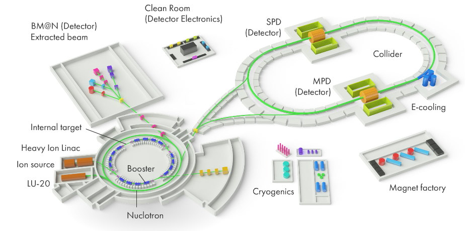
Figure 1. NICA complex with the BM@N experiment at the extracted Nuclotron beam

The physics program of the BM@N experiment includes the study of the equation of state of dense nuclear matter, the production of strange mesons and (multi-)strange hyperons close to the kinematic threshold, the search for hypernuclei, in-medium effects for strangeness and vector mesons, collective flows, polarization and femtoscopy of hadrons. Particle yields, ratios, transverse momentum spectra, rapidity and angular distributions, as well as fluctuations and correlations of hadrons are studied as a function of the collision energy and centrality.

In collisions of bismuth ions with heavy targets at these energies, very high multiplicity can be reached, and the BM@N facility should identify the produced particles with high efficiency and estimate their parameters with high precision. For this purpose, BM@N combines high precision track measurements in the magnetic field with the time-of-flight particle identification and the measurements of the forward spectator detectors for the event characterization (centrality and reaction plane).

The BM@N setup in Run 9 is shown in figure 2. Upstream of the target, the beam ions pass through the beam counters BC1 and BC2 with the veto counter VC, the Silicon Beam Tracker (SiBT) and the silicon beam profilometers (SiProf). The target is surrounded by the Barrel Detector (BD) used in the trigger. The central tracking system located inside the large-aperture analyzing dipole magnet consists of the Vertex Silicon Plane (VSP), the Forward Silicon Detector (FSD) and the Gas Electron Multiplier (GEM) stations, and it is followed by the Fragment Detector (FD). The outer tracking system includes four small and two large Cathode Strip Chambers (CSC) and the Drift Chambers (DCH, not used since Run 9); the time-of-flight systems TOF-400 and TOF-700 are used for the particle identification. The forward detectors – the Scintillation Wall (ScWall), the Forward Quartz Hodoscope (FQH) and the Forward Hadron Calorimeter (FHCal) – determine the collision centrality and the reaction plane, and the Highly Granular Neutron Detector (HGND) measures neutrons.

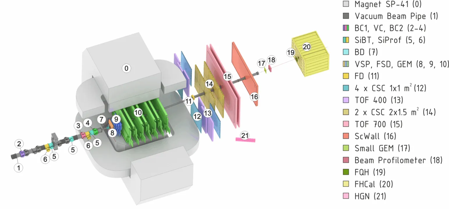
Figure 2. Scheme of the BM@N setup in Run 9

1.2 Purposes of the BmnRoot framework

The software and computing parts of the BM@N project are responsible for the activities including design, evaluation and calibration of the detector; storing, access, reconstruction and analysis of the data; and development and maintenance of a distributed computing infrastructure for physicists engaged in these tasks. To support the BM@N experiment, the software framework BmnRoot has been developed. It provides a powerful tool for detector performance studies, event simulation, and development and usage of algorithms for reconstruction and physics analysis of data of the fixed target events registered by the BM@N facility. The BmnRoot is implemented in the programming language C++ and based on the ROOT environment and the object-oriented framework FairRoot (developed for the experiments of the FAIR facility at GSI).

The flexibility of the framework is gained through its modularity. The physics and detector parts could be written by different groups. In the applied framework, the detector response simulated by a package currently based on the Virtual Monte Carlo concept allows switching simulation between different transport packages without changing the user code (at present, Geant4 is mainly used). For a realistic simulation of various physics processes, an interface to the event generators for nuclear collisions, e.g., UrQMD, DCM-SMM, DCM-QGSM and PHSD, is provided. One can easily choose between different modules, e.g., event generators. The same framework – BmnRoot – is used to define the experimental setup and provides simulation, reconstruction and physics analysis of simulated and experimental data. Using the same internal structure, the user can compare easily at any time the real data with the simulation results.

Experimental data of the BM@N runs are processed in the same framework: raw data files written by the Data Acquisition System are converted to the ROOT format and decoded to detector digits, which are then reconstructed by the same reconstruction chain as the simulated ones, so that simulated and experimental DST files have a common format. The parameters of the runs and detectors are taken from the Unified Condition Database (UniConDa), and the setup geometry – from the Geometry Database.

The BmnRoot environment also includes the tool for event navigation, inspection and visualization. The BM@N event display for Monte Carlo and experimental data is based on the EVE (Event Visualization Environment) package of the ROOT. The event display macro can be used to display both Monte Carlo tracks and their points, and reconstructed hits, tracks and energy deposited in calorimeter towers, together with the BM@N detector geometry, both offline and online during the runs. The Event Manager implemented in the framework delivers an easy way to navigate through the event tree and to make cuts on energy, particle PDG codes, etc. in selected events.

In addition, BmnRoot includes the interfaces to the information systems of the experiment (the Unified Condition Database, the Geometry Database, the Electronic Logbook, the Event Metadata System and others), the Online Histogramming System for monitoring of the data quality during the runs, the tools for the alignment of the tracking detectors and for the quality assurance of the simulation and reconstruction, as well as the NICA-Scheduler for the distributed data processing on computing clusters.

1.3 Points of Contact

Dr. Gertsenberger Konstantin, Software Coordinator of the BM@N experiment
Email: gertsen@jinr.int

BM@N Collaboration (bmn.jinr.int)
Veksler and Baldin Laboratory of High Energy Physics
Joint Institute for Nuclear Research, Dubna

BM@N Forum, Software section: bmn-forum.jinr.int
BM@N Wiki: bmn-wiki.jinr.int
BM@N Project Management System: bmn-pm.jinr.int

1.4 Organization of the Guide

1: General Information

This section contains general information about the BM@N experiment and the BmnRoot environment, including the purposes, points of contact, and acronyms and abbreviations.

2: Installation

The second section briefly describes the external packages required by BmnRoot – FairSoft and FairRoot – and refers to the up-to-date installation instructions of the BmnRoot framework.

3: BmnRoot Structure

This section contains the information about the structure of the BmnRoot framework, and briefly describes its directories and macros to be executed in the ROOT environment.

4: Simulation, Reconstruction and Analysis Tasks

The fourth section details the main macros of the BM@N data processing chain: simulation (run_sim_bmn.C), decoding of the experimental raw data (run_raw_bmn.C), event reconstruction (run_reco_bmn.C) and physics analysis (run_ana_bmn.C). It also lists event generators and transport packages which can be used.

5: Event Display of the BM@N Experiment

This section introduces the ROOT geometry package and presents the event display system intended to visualize the detector geometries and events of particle collisions with the fixed target, both simulated and experimental (offline and online), its structure, options and features as well as integration into the BmnRoot software.

6: Information Systems of the BM@N Experiment

The section describes the information systems of the experiment used in the BM@N data processing – the Unified Condition Database, the Geometry Database, the Electronic Logbook, the Event Metadata System, the Data Management System and the Slow Control Viewer – and their interfaces in BmnRoot.

7: Distributed Computing

This section describes the data processing pipeline of the experiment and the computing platforms used for storing and processing of the BM@N data – the DAQ Data Center (DDC), the NICA cluster, the MLIT CICC complex and the HybriLIT platform with the Govorun supercomputer – as well as the distributed data storage, batch systems and the NICA-Scheduler simplifying parallel processing of the BM@N data.

8: BmnRoot Development

The section describes the development of BmnRoot: the access to the GitLab repository, the use of the Git version control system with own branches and merge requests, the automatic testing and deployment of new versions, and the coding conventions: code formatting, naming, comments and documentation, code organization and the DRY principle.

9: Frequently Asked Questions

The last section contains answers to frequently asked questions on working with BmnRoot.

1.5 Acronyms and Abbreviations

• BM@N – Baryonic Matter at Nuclotron, the fixed target experiment of the NICA facility.
• CVMFS – CernVM File System used for the distribution of the experiment software.
• DAQ – Data Acquisition System of the experiment.
• DMS – Data Management System of the experiment.
• DST – Data Summary Tape, the format of files with reconstructed data used in physics analysis, see the BmnRoot DST Format document.
• e-Log – Electronic Logbook of the experiment.
• EMS – Event Metadata System of the experiment.
• EOS – distributed file system developed at CERN, which is used for the storage of the BM@N data.
• JINR – Joint Institute for Nuclear Research, Dubna.
• Macro – “small” C++/ROOT program code executed by the ROOT C++ interpreter (Cling).
• MC – Monte Carlo (simulated data).
• MLIT – Meshcheryakov Laboratory of Information Technologies of JINR.
• NICA – Nuclotron-based Ion Collider fAcility at JINR.
• ROOT – modular scientific software framework, born at CERN, to deal with data processing, statistical analysis, visualization and storage in the research on high-energy physics.
• Run, run – in this document, Run with the capital letter means a session of the BM@N experiment (e.g. Run 9 is the last one), also called run period, whereas run with the small letter means a separate data taking run (usually about 30 minutes) within the session.
• SCS – Slow Control System of the experiment.
• SLURM – batch system distributing user jobs on the nodes of computing clusters.
• UniConDa – Unified Condition Database of the BM@N experiment.
• VMC – Virtual Monte Carlo, interface to the particle transport packages.

2. Installation

2.1 FairSoft Package

Many physics packages are necessary for the BmnRoot environment. Some of them can be installed using the package manager of the Linux distribution, but many others have to be installed from sources. To make the installation procedure as easy as possible an additional package called FairSoft is provided by the FAIR collaboration. This package takes care of the installation of needed programs in the right order and with the right compilation flags. In the end, libraries and packages included in the FairSoft are installed in one directory.

The FairSoft package takes care of downloading, configuring, building and installing all required external software in the right order and with consistent compilation flags. Different FairSoft releases contain different versions of the packages, therefore the installation instructions of BmnRoot specify the FairSoft release to be used with the current BmnRoot version.

The FairSoft package includes, in particular, the following packages:

• ROOT 6 – the data processing framework of CERN;
• Geant4 with its data files and Geant3 – the particle transport packages;
• VMC, Geant4_VMC and VGM – the Virtual Monte Carlo interfaces and geometry converters;
• Pythia6 and Pythia8 – event generators of high-energy physics, also used for particle decays;
• HepMC and CLHEP – event record and class library for high-energy physics;
• FairLogger – the logging library used by FairRoot and BmnRoot;
• Boost, fmt, yaml-cpp, XercesC, ZeroMQ and other general-purpose libraries.

The FairSoft package can be found on the GitHub repository.

2.2 FairRoot Framework

FairRoot is an object-oriented simulation, reconstruction and data analysis framework developed at GSI for the experiments of the FAIR facility (Darmstadt, Germany) and used by a number of other experiments, including the experiments of the NICA project. It is based on ROOT and the Virtual Monte Carlo concept, and provides the base classes for the main tasks of event data processing, so the software of an experiment implements only experiment-specific parts, such as detector descriptions and data processing algorithms.

FairRoot is installed as a separate external package on top of FairSoft, and BmnRoot is built against it: the path to the FairRoot installation is set by the FAIRROOTPATH environment variable. The main FairRoot classes used in BmnRoot are the following:

• FairRunSim – manager of a simulation run: modules of the setup geometry (FairModule, FairDetector), event generators (FairPrimaryGenerator), magnetic field (FairField) and the particle transport package;
• FairRunAna – manager of a reconstruction or analysis run executing a list of tasks for each event;
• FairTask – base class of all processing tasks: digitizers, hit and track finders, analysis tasks;
• FairRootManager – input/output manager providing access to the branches of the input data and registering the output branches;
• FairSource, FairSink – input source and output sink of the event data, e.g. FairFileSource and FairRootFileSink;
• FairRuntimeDb – runtime database of parameter containers, e.g. FairGeoParSet with the setup geometry;
• FairLogger – logging system with severity levels used by the LOG(info), LOG(error), etc. macros.

In addition, FairRoot provides templates – the starting points for implementation of different modules, which are located in the templates directory of the FairRoot repository:

• NewDetector_root_containers, NewDetector_stl_containers – a new detector for the Monte Carlo simulation storing MC points in ROOT containers (TClonesArray, as in BmnRoot) or in std::vector (Section 9.2);
• NewTask – a new task, e.g. a digitizer, reconstruction or analysis task (Section 9.1);
• NewParameterContainer – a new parameter container with reading and writing of the parameters;
• TimeBased – classes for time-based simulation (buffer, sorter);
• project_root_containers, project_stl_containers – a new project with base implementations of generators, geometries, magnetic field, data classes, detector classes and macros.

Each template includes the rename.sh script, which renames the template classes and files according to the given name. Detailed information on FairRoot can be found at the FairRoot GitHub repository.

2.3 BmnRoot Installation

The installation procedure of BmnRoot depends on the operating system and on the versions of the external packages, and it is updated together with the software. Therefore, the up-to-date installation instructions, including the required system packages, the recommended FairSoft and FairRoot releases and the configuration options, are maintained on the BM@N website in the Software Installation section.

The source code of BmnRoot is stored in the GitLab repository of JINR (https://git.jinr.ru/nica/bmnroot); the default development branch is dev.

BmnRoot is built with CMake in a separate build directory. During the configuration, CMake generates the config.sh script in the build directory, which sets all environment variables required to work with BmnRoot: paths to ROOT, FairSoft and FairRoot (ROOTSYS, SIMPATH, FAIRROOTPATH), the main BmnRoot directory (VMCWORKDIR), the location of the Geometry Database (DBL_FILE_PATH, GEOMPATH), the data paths of the transport packages, as well as the PATH, LD_LIBRARY_PATH and ROOT_INCLUDE_PATH variables. BmnRoot macros do not work without this environment, so the script has to be executed in every new terminal (bash) before running ROOT:

source <BmnRoot build directory>/config.sh

On the JINR computing clusters, pre-built versions of FairSoft, FairRoot and BmnRoot for the supported operating systems are available in the CVMFS repository /cvmfs/bmn.jinr.ru.

The access to the source code of BmnRoot, its development with Git, the automatic testing of the changes and the coding conventions are described in Section 8.

3. BmnRoot Structure

3.1 BmnRoot Directories

BmnRoot is based on the ROOT environment and the FairRoot framework (Section 2.2), which provide the base classes for simulated and experimental data processing. The top directory of the BmnRoot framework contains the following main directories:

• base – base classes of BmnRoot: data containers of digits, hits, tracks and MC information (base/data), headers of the output files (base/header), raw data classes (base/raw), math tools and input sources;
• cmake – CMake modules and scripts to build the BmnRoot software;
• config – common configuration files for fine-tuning of the data processing and visualization, e.g. the configuration of the raw data converter and decoder (bmnconf.json);
• database – C++ interfaces to the information systems of the experiment: Unified Condition Database (uni_db, Section 6.1), Geometry Database (geo_db, Section 6.2), Electronic Logbook (elog_db, Section 6.3), Event Metadata System (event_db, Section 6.4), Data Management System (file_db, Section 6.5) and the Slow Control Viewer (tango, Section 6.6);
• decoder – Raw Data Decoder converting the raw data of the BM@N runs to the ROOT format and decoding them to detector digits (Section 4.4);
• detectors – classes for simulation and hit reconstruction of the BM@N subdetectors, one subdirectory per detector, e.g. SiBT, bd, vsp, silicon, gem, csc, dch, tof1 (TOF-400 and TOF-700), fhcal, scwall, hodo, ndet;
• eventdisplay – classes for visualization of the detector geometry and collision events (Section 5);
• field – classes of the magnetic field: constant field or field defined by a map file;
• gconfig – macros and files to steer the simulation: cuts, physics lists, settings of the Geant3 and Geant4 transport packages;
• generators – interfaces to the event generators (Section 4.2);
• geometry – geometry files of the BM@N subdetectors in ROOT (.root) and ASCII (.geo) formats; the setup geometries used in the data processing are taken from the Geometry Database (Section 6.2);
• input, parameters – text files with detector mappings, calibrations and other parameters used in the data processing;
• macro – ROOT macros for simulation, reconstruction and physics analysis of the BM@N data (Section 3.2);
• monitor, online – Online Histogramming System for monitoring of the data quality and online processing of the data during the BM@N runs;
• physics – physics analysis tasks and related tools, including the BmnAnalysisTask template (Section 4.6);
• QA – classes for quality assurance (QA) histograms of the simulation and reconstruction;
• reconstruction – classes of the event reconstruction: Kalman filter (KF), inner tracking (tracking), global tracking (globaltracking), particle identification (identification), forward detectors (fhcal, scwall, hodo, ndet), centrality determination (centrality) and filling of the DST (dst);
• alignment, align_new – alignment of the BM@N tracking detectors;
• services – auxiliary tools, including the NICA-Scheduler (nica_scheduler, Section 7.7) and scripts for code formatting and testing.

The top directory of the BmnRoot framework also includes the following files:

• CMakeLists.txt – the main CMake script to build BmnRoot;
• README.md – short description of the BmnRoot software with links to the installation instructions and support resources;
• COPYING – license of BmnRoot;
• SetEnv.sh – bash script setting the paths to FairSoft and FairRoot (SIMPATH, FAIRROOTPATH) for the initial CMake configuration of BmnRoot (Section 2.3).

3.2 BmnRoot Macros

Macro is the main executable element of the BmnRoot environment. Usually, it has .C extension. How to run a macro with the ROOT C++ interpreter (Cling), you can find in the ROOT documentation. Most of the BmnRoot macros are located in the macro directory. It includes the following subdirectories:

• run – main macros of the BM@N data processing chain (see below);
• detectors – macros to check the data processing of separate subdetectors;
• eventdisplay – event display macro to graphically present the BM@N geometry and collision events (Section 5);
• geometry – macros for creating files with subdetector geometries in ROOT format;
• howTo – examples of working with BmnRoot data, e.g. readDst.C for reading DST files;
• magfield – macros to create and work with the magnetic field maps of the experiment;
• physics – macros for physics analysis of the BM@N data;
• raw – macros to work with the Raw Data Decoder;
• alignment, globaltracking, recotools, embedding – macros for alignment, global tracking tests, reconstruction tools and embedding;
• monitor – macros and files to run the Online Histogramming System;
• profiling – files for profiling the main BmnRoot macros and checking them for memory leaks.

The main macros and subdirectories of the macro/run directory are listed below:

• run_sim_bmn.C – simulation of BM@N events for the selected event generator (Section 4.3);
• run_raw_bmn.C – conversion of the experimental raw data to the ROOT format and their decoding to detector digits (Section 4.4);
• run_reco_bmn.C – reconstruction of simulated and experimental BM@N events (Section 4.5);
• run_ana_bmn.C – physics analysis of the reconstructed simulated and experimental events (Section 4.6);
• QA – macros to create QA histograms for the BM@N simulation and reconstruction.

One can start to learn BmnRoot with the run_sim_bmn.C and run_reco_bmn.C macros, and then process the obtained DST file with run_ana_bmn.C. These macros are described in the next section in details.

4. Simulation, Reconstruction and Analysis Tasks

4.1 Virtual Monte Carlo

Basically, there are two ways to simulate the behavior of a system: either one can describe its evolution analytically, in which case computers are used to find the solution of the dynamic equations, or a probabilistic approach is used, in which at each step pseudo-random numbers are used to select one among different physics processes. Example of the first approach is the computation of charged particle paths inside a magnetic field. When dealing with the interactions of particles with matter, the second approach is usually followed, because of the variety of possible physics processes and of their discrete nature. Because such approach is based on pseudo-random numbers, it is usually called a "Monte Carlo" method.

TVirtualMC class of the ROOT environment provides a virtual interface to Monte Carlo applications, allowing the user to build a simulation independent of any actual underlying Monte Carlo implementation itself. A user will have to implement a class derived from the abstract Monte Carlo application class. The concrete Monte Carlo implementation such as Geant3 or Geant4, is selected at run time – when processing a ROOT macro where the concrete Monte Carlo object is instantiated. This allows for comparison between different engines (necessary to estimate the theoretical uncertainties) using a single application.

Monte Carlo simulations always have to describe the input particles, together with their interactions, and the detector (geometry, materials and read-out electronics). The definition of particles, available interactions and detector is carried on during the initialization phase. The main body of the application is then a loop over all particles that are traced through all materials until they exit, stop or disappear (by decay or annihilation). The tracing is done in a discrete fashion: at each step, the detector volume is found in which the particle is located and pseudo-random numbers are used to "draw" one among possibly several physical processes, to simulate the interaction of the particle with the matter. If an interaction occurs, the energy lost by the particle is computed and subtracted from its kinetic energy. When the latter reaches zero, the particle stops in such volume, otherwise a new step is performed.

Having computed the energy lost by all particles inside the detector, one has to simulate the behavior of the read-out electronics. This is usually done later, with another program that receives the energy lost in different locations as input, but it can also be done by the very same application that is performing the particle tracing inside the detector. Usually, the simulation of the read-out electronics also involves some use of pseudo-random generators, at least to simulate the finite resolution of any real measuring device.

The Virtual Monte Carlo (VMC) allows to run different simulation Monte Carlo without changing the user code and therefore the input and output format as well as the geometry and detector response definition. It provides a set of interfaces, which completely decouple the dependencies between the user code and the concrete Monte Carlo. The implementation of the TVirtualMC interface is provided for two Monte Carlo transport codes, Geant3 and Geant4. The implementation for the third Monte Carlo transport code, Fluka, has been discontinued. The VMC is now fully integrated with the ROOT geometry package TGeo, and users can easily define their VMC application with TGeo geometry definition (figure 3).

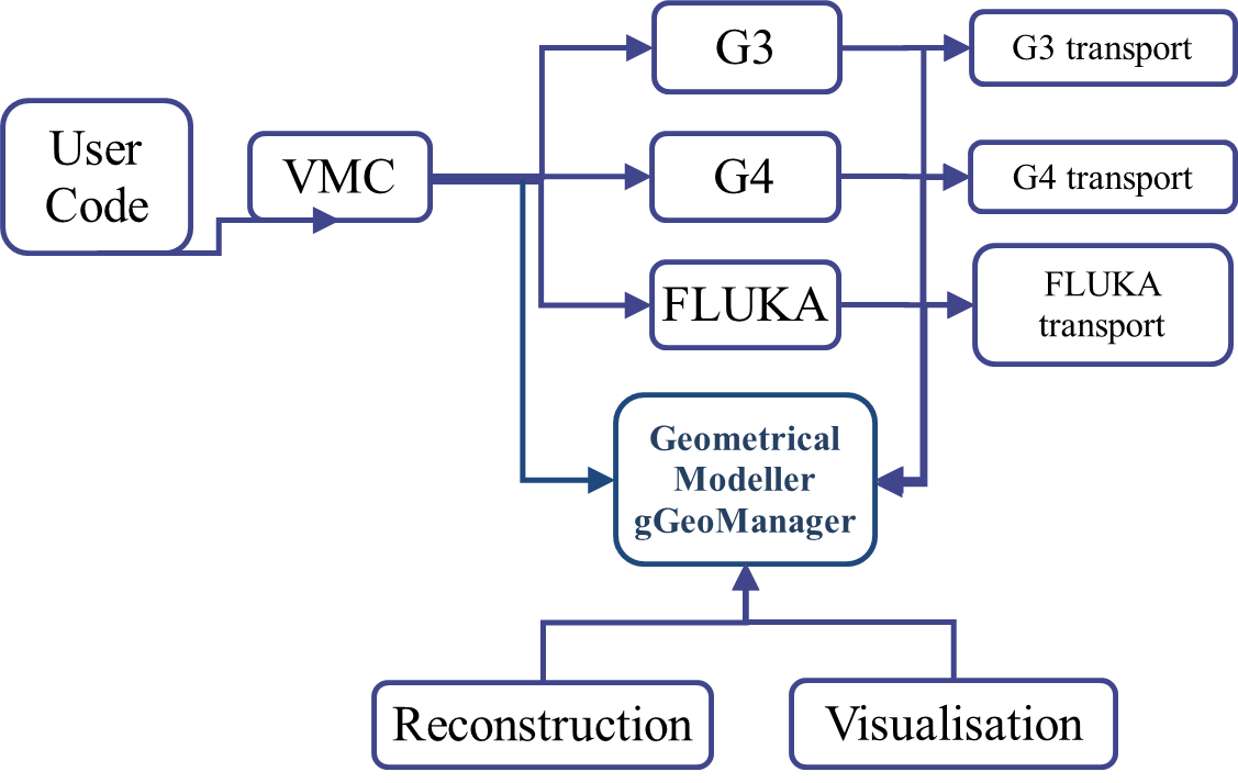
Figure 3. Geometrical Modeller (gGeoManager) for the MC simulation

4.2 Event generators

Event generators are software libraries that randomly generate high-energy particle physics events. Monte Carlo (because they exploit Monte Carlo methods) event generators are essential components of experimental analyses today and are also widely used by theorists and experiments to compare experimental results with theoretical predictions and to make predictions and preparations for future experiments.

Monte Carlo generators allow to include theoretical models, phase space integration in multiple dimensions, inclusion of detector effects, and efficiency and acceptance determination for new physics processes. All event generators split the simulation up into a set of phases, such as initial-state composition and substructure, the hard process, parton shower, resonance decays, multiple scattering, hadronization and further decay. As a result, event generator produces the final-state particles, which feed into the detector simulation, allowing a precise prediction and verification for the entire experimental setup.

The BmnRoot framework supports an extended set of event generators (physics models) for particle collisions, which are commonly used in HEP experiments, such as:

• Ultrarelativistic Quantum Molecular Dynamics (UrQMD);
• Dubna Cascade Model with Statistical Multifragmentation Model (DCM-SMM);
• Dubna Cascade Model – Quark-Gluon String Model (DCM-QGSM, LAQGSM);
• Parton-Hadron String Dynamics (PHSD, HSD);
• 3-Fluid Dynamics (3FD) and hybrid vHLLE+UrQMD model;
• Pluto event generator;
• any generator, whose output is converted to the UniGen format;
• simple generators of FairRoot: box generator of particles in given momentum and angle ranges (FairBoxGenerator), single particle (FairParticleGenerator) and ion (FairIonGenerator) generators.

Files of different event generators are located on the NICA cluster in the /eos/nica/bmn/sim/gen directory, e.g. /eos/nica/bmn/sim/gen/DCMSMM.

Figure 4 shows the place of the event generators in the data processing chain and the further steps of simulation in particle physics.

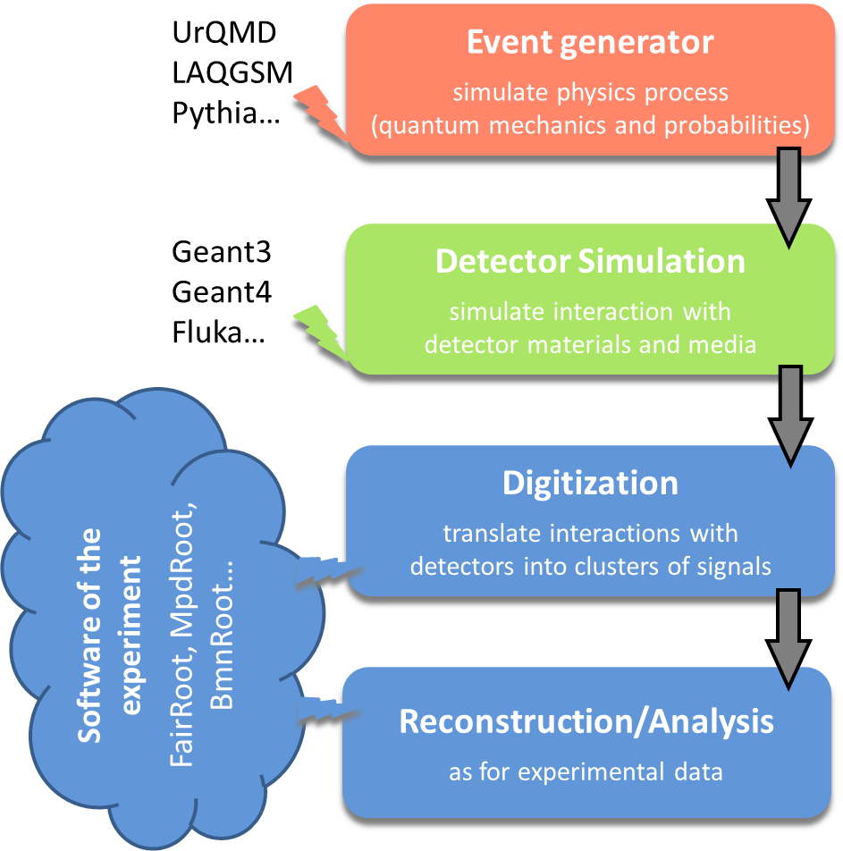
Figure 4. Simulation and analysis steps of high energy physics experiment

Partly due to historic reasons, many event generators are written in Fortran, newer ones are usually implemented in C++ language. Most particle collision (event) generators produce files of own format, which is then used in simulation of the experiment. Figure 5 presents the steps above with file storage levels of the BmnRoot in more details.

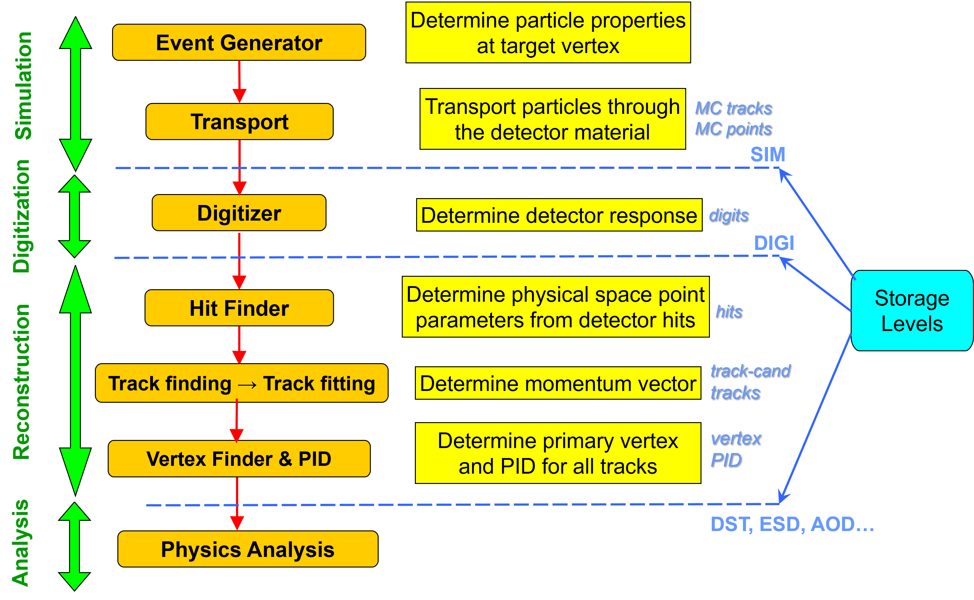
Figure 5. Data processing steps and storage levels of the BM@N experiment

4.3 Simulation of the BM@N experiment

BM@N simulation includes interactions and particles of interest, geometry of the system, materials used, generation of test events of particles, interactions of particles with matter and electromagnetic fields, response to detectors, records of energies and tracks, analysis of the full simulation at different detail and visualization of the detector system and collision events. As the events are processed via the simulation, the information is disintegrated and reduced to that generated by particles when crossing a detector.

Simulation in high energy physics experiments uses transport packages to move the particles through experimental setup from initial state or origin files produced by event generators, such as UrQMD or DCM-SMM described above. Geant (short from “geometry and tracking”) transport package is developed at CERN and most commonly used today. Geant3 was implemented in Fortran programming language, whereas Geant4 is developed in C++.

Transport includes detailed description of detector geometries and propagates all particle tracks through detector materials and media. The detector geometries are described by Geant and native geometrical models. During tracking of all particles through detectors, the energy losses of the particles in the sensitive volumes are stored as MC points, which are then converted to the detector responses (digits) used in the reconstruction. In order to evaluate the software and detector performance, simulated events are processed through the whole cycle and finally the reconstructed information about particles is compared with the information taken directly from the Monte Carlo generation.

To simulate the passage of particles through the detectors, a directory is created for each subdetector system in the detectors directory (e.g. detectors/silicon). It describes the logic of processing the particles crossing the detector. The detector class derived from FairDetector (e.g. BmnSilicon) defines the sensitive volumes and stores the steps of the particles in them as MC points (BmnSiliconPoint), and the digitizer (BmnSiliconDigitizer) converts the MC points into the detector digits. The basic template of such a detector description can be taken from FairRoot, as described in the FAQ (Section 9.2).

To simulate BM@N events of particle collisions with a fixed target, the run_sim_bmn.C macro is used. The macro transports primary particles produced by an event generator through the BM@N setup and converts the obtained MC points into detector digits, so that the output file contains both Monte Carlo information and the simulated detector responses.

Function parameters of the macro run_sim_bmn.C:

Parameter	Description
TString genFile	Path to the input file of the event generator, if required by the selected generator (it is not used by the BOX, PART and ION generators). Default: ""
TString simFile	Path to the result file with the simulated data; the directory of the file is created, if it does not exist. Default: $VMCWORKDIR/macro/run/bmnsim.root
Int_t nStartEvent	Number (starting with zero) of the first event in the generator file to be transported. Default: 0
Int_t nEvents	Number of events to transport; for the generators reading input files, 0 means all events of the file starting with nStartEvent. Default: 10
enumGenerators generatorName	Event generator: UNIGEN, URQMD, QGSM, HSD, BOX, PART, ION, DCMQGSM or DCMSMM. Default: BOX
TString geometryTag	Tag of the BM@N setup in the Geometry Database; a tag prefix followed by ‘:’ means the latest approved setup of the run period. The tag can be followed by ‘;’ and a path to an XML file with a local customization of the setup geometry (Section 6.2.3). Default: "run9:"
Bool_t saveGeoInfo	Whether to store particle trajectories (GeoTracks branch) for the event display and to save the full setup geometry to the additional full_geometry.root file. Default: kFALSE
Bool_t useRealEffects	Whether to take into account realistic effects (Lorentz shift, misalignment) in the digitizers of the strip detectors. Default: kTRUE

Examples of running the simulation with the BOX generator (100 events, the latest Run 9 setup) and with a DCM-SMM file of Xe + CsI collisions:

root -b -q '$VMCWORKDIR/macro/run/run_sim_bmn.C("", "bmnsim.root", 0, 100)'
root -b -q '$VMCWORKDIR/macro/run/run_sim_bmn.C("<path>/DCMSMM_XeCsI_3.9AGeV_mb_10k_116.r12", "bmnsim.root", 0, 1000, DCMSMM, "run9:")'

The main macro lines are described below. On the first step (after creating a timer for execution profiling), the simulation macro creates the FairRunSim (run simulation) class and chooses a transport package for it. Geant4 is used by default; to switch to Geant3, change the name of the engine:

fRun->SetName("TGeant4");   // or "TGeant3"

This function also automatically runs ROOT macros from the gconfig directory to set the configuration of the selected transport package. On the next step, the BM@N setup geometry is loaded from the Geometry Database by the GeoSetup class (Section 6.2). A tag ending with ‘:’ (e.g. "run9:") is replaced by the tag of the latest approved setup of the run period, and the period number is used to select the detector configurations in the digitizers:

GeoSetup gSetup;
// "run9:" tag -> the latest approved setup of Run 9, e.g. run9_26.09.0
geometryTag = gSetup.GetLastApprovedSetupTag("run9").c_str();
// xmlFile - optional path to an XML file with a local customization
gSetup.LoadSetupToFairRunSim(geometryTag.Data(), xmlFile);

Then the event generator is defined. The FairPrimaryGenerator class combines the generators, and the beam parameters (position and angular spread of the beam, target position and thickness) are set for it to smear the position of the primary vertex:

FairPrimaryGenerator* primGen = new FairPrimaryGenerator();
fRun->SetGenerator(primGen);
primGen->SetBeam(beamX0, beamY0, beamSigmaX, beamSigmaY);
primGen->SetTarget(targetZ, targetDz);

The generator is selected by the generatorName parameter. The generators reading input files (UrQMD, DCM-SMM, DCM-QGSM, PHSD, UniGen) use the genFile path, whereas the parameters of the simple BOX, PART and ION generators (particle type, multiplicity, momentum and angle ranges) are set directly in the macro. If you do not have access to generator files, you can use the BOX generator to propagate selected particles in the desired directions.

The beam particle, target and beam energy are parsed from the name of the generator file, e.g. DCMSMM_XeCsI_3.9AGeV_mb_10k_116 means Xe beam, CsI target and 3.9 GeV per nucleon. They are written to the FairBaseParSet container of the output file (the beam energy – to the beam momentum field fBeamMom, the beam and target – to the container description as “beam;target”) and used later to fill the run header of the DST file. The scale of the magnetic field map from the Geometry Database is defined by the beam energy (the default scale corresponds to 3.8 GeV per nucleon):

BmnFieldMap* magField =
    dynamic_cast<BmnFieldMap*>(gSetup.GetMagneticField(fieldScale));
fRun->SetField(magField);

The energy losses of particles in the sensitive volumes (MC points) are converted to the detector responses – digits – by digitizer tasks added to FairRunSim, one for each subdetector: SiBT, SiProf, BD, SiMD, VSP, Silicon, GEM, CSC, FHCal, ScWall, Hodo and Ndet, for example:

BmnGemStripDigitizer* gemDigit = new BmnGemStripDigitizer(run_period);
gemDigit->SetUseRealEffects(useRealEffects);
fRun->AddTask(gemDigit);

The next function initializes the BM@N simulation, i.e. the Virtual Monte Carlo classes and tasks: fRun->Init(). To run event simulation, the following line is executed: fRun->Run(nEvents). In addition, the radiation length manager can be enabled by fRun->SetRadLenRegister(kTRUE): the FairRadLenManager class determines the particle fluency through the volume boundaries to estimate the radiation length data and the material budget of the setup.

Figure 6 presents the main modules of the BmnRoot framework and their relationship during the simulation.

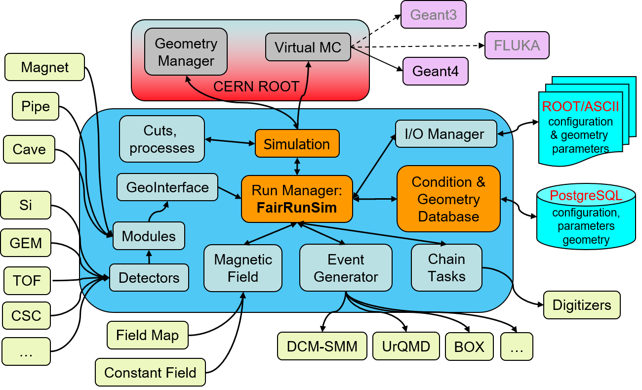
Figure 6. The scheme of the BmnRoot modules in the simulation

The input/output manager (FairRootManager, shown on the figure as I/O manager) provides access to the branches of the input data and registers the output branches, the event data are stored in ROOT trees. The Runtime Parameter Manager (FairRuntimeDb) is the manager class for all parameter containers: it includes the container factories, the list of parameter containers and the list of runs. The parameter containers are requested by the tasks in their SetParContainers() function and initialized from ROOT or ASCII parameter files set in the macro.

Subdetector geometries can be defined using different input formats: ASCII or ROOT files (ROOT Geometry format presented in the form of TGeoVolumes tree) or defined directly in the source code (non-recommended). In BmnRoot, the detector geometries are stored in the ROOT format, whereas the ASCII format is used for the cave, media and some passive volumes, such as the target. The ASCII input format for detector geometry consists of volumes defined by the following sequence:

	Example
Volume name	target
Mother volume name	pipe_vac_1
Shape name	TUBE
Medium name	Gold
Shape parameters	0. 0. -0.25 0. 2.5 0. 0. 0.25
Positioning of the volume in a mother node: position and rotation matrix	0. 0. 0. 1. 0. 0. 0. 1. 0. 0. 0. 1.

The simulation result is the bmnsim.root (default name) file. Its event tree bmndata contains MC tracks (MCTrack branch), MC points of the subdetectors (branches <Detector>Point, e.g. SiliconPoint), their digits (e.g. BmnSiliconDigit), the MC event header (MCEventHeader.) and, if saveGeoInfo is set, the particle trajectories (GeoTracks). The file also includes the magnetic field parameters (BmnFieldPar) and the BM@N setup geometry stored in the FairGeoParSet container with the geometry tag in its description, which is presented by the ROOT geometry manager gGeoManager (TGeoManager class). To get the geometry from this file, you can execute the following lines in a stand-alone ROOT macro:

TFile* f = new TFile("bmnsim.root");
f->Get("FairGeoParSet");   // and then use gGeoManager

ROOT Geometry package is described in the Section 5.1. ROOT files are created via the object streaming mechanism (information about ROOT Streamers you can find in the ROOT documentation) and are presented by a tree of objects.

4.4 Decoding of the experimental raw data

Experimental data of the BM@N experiment are written by the Data Acquisition System (DAQ) to raw files in a binary format (files with the .data extension, e.g. run_Top_9696_ev2_p25.data). Before the reconstruction, the raw data have to be converted to the ROOT format and decoded to detector digits – the same data level as the output of the digitizers in the simulation. This step is performed by the run_raw_bmn.C macro, which drives the Raw Data Decoder (BmnRawDataDecoder class) through two steps:

1. conversion of the binary raw file into an intermediate RAW ROOT file containing the digits of the readout electronics (ADC, TDC, TQDC, synchronization data, etc.);
2. decoding of the RAW ROOT file into detector digits using the mapping and calibration files selected for the given run period, run number and setup.

Function parameters of the macro run_raw_bmn.C:

Parameter	Description
TString file	Full path to the input file: the raw .data file (todo = 1 or 2) or the intermediate RAW ROOT file (todo = 0). Default: ""
TString outfile	Full path to the result file with detector digits; if it is empty, the file name is built as bmn_run<run number>_evXX_pXX_digi.root. Default: ""
Long_t nEvents	Number of events to process, 0 means all events. Default: 0
UInt_t period	BM@N run period number to pick up the mapping and calibration files. Default: 8
UInt_t todo	Processing mode: 0 – decoding of a RAW ROOT file to digits, 1 – conversion and decoding of a raw file to digits, 2 – conversion of a raw file to the RAW ROOT file only. Default: 1
Bool_t doHoldRawRoot	If kFALSE, the intermediate RAW ROOT file (bmn_run<run number>_evXX_pXX_raw.root) is deleted after the decoding. Default: kTRUE

The run number is read from the raw data. The set of detectors to be decoded is defined in the macro by the map of DetectorId flags (kGEM, kSILICON, kTOF1, kFHCAL, etc.), the general parameters of the converter and decoder are read from the $VMCWORKDIR/config/bmnconf.json file, and the mapping and calibration files of the detectors, located in the input directory, are set for the decoder by names, which include the period number, for example:

// e.g. GEM_map_run9.txt and FHCAL_map_period9.txt for period 9
decoder->SetGemMapping(TString("GEM_map_run") + PeriodSetupExt);
decoder->SetFHCalMapping(TString("FHCAL_map_period") + PeriodSetupExt);

If the SetTof400Mapping line is commented out, the TOF-400 maps are read from the Unified Condition Database.

The result digit file contains the event tree bmndata with the event header (BmnEventHeader. branch: run and event numbers, event time, trigger information), the digit branches of the subdetectors (e.g. VSP, SILICON, GEM, CSC, TOF400, TOF701, FHCalDigi, ScWallDigi, HodoDigi, NdetDigi) and the digits of the trigger and beam counters, the tree with spill information, as well as the run header (DigiRunHeader) and the metadata of the raw file. Example of the conversion and decoding of a raw file of Run 9:

root -b -q '$VMCWORKDIR/macro/run/run_raw_bmn.C("run_Top_9696_ev2_p25.data", "", 0, 9)'

The macro creates the intermediate bmn_run9696_ev2_p25_raw.root file and the bmn_run9696_ev2_p25_digi.root file with detector digits, which is then processed by the reconstruction macro described in the next subsection.

4.5 BM@N event reconstruction

Event reconstruction is the process of interpreting the electronic signals produced by the detector to determine the original particles that passed through, their momenta, directions, and the primary vertex of the event. Event reconstruction consists of the following main steps:

• hit reconstruction in subdetectors;
• track reconstruction usually composed of:
  • searching for track candidates in the main tracker;
  • track propagation, e.g., using the Kalman filter;
  • matching with other detectors (global tracking);
• vertex finding;
• particle identification.

The tasks for charged-track reconstruction in high energy physics are pattern recognition (i.e., track finding) and track fitting. The common approach to the track reconstruction problem is based on the Kalman filtering technique. The multiple scattering can also be handled properly by the method. The Kalman filter is a set of mathematical equations that provides an efficient computational (recursive) solution of the least-squares method. The algorithm starts from track candidates (“seeds”), for which vectors of initial parameters and covariance matrices are evaluated. Then each track is propagated to some surface (detector or intermediate point). The new covariance matrix can be obtained using the Jacobian matrix of the transformation, i.e., the matrix of derivatives of propagated track parameters with respect to current parameters.

In BmnRoot, the inner tracks are found by default by the vector finder (VectorFinder) based on the cellular automaton approach: the hits of neighbouring stations are combined into doublets and triplets (track segments) selected by windows in the track slopes and curvature, which are then extended station by station with the Kalman filter. The search is performed in several passes with the decreasing minimal number of hits, and duplicated and fake tracks are rejected, also by a BDT classifier. Alternatively, the CellAuto tracking used before can be selected, and the L1 (CBM) tracking is planned to be used for the online tracking.

Simulated (MC) tracks are described by the particle code (integer “PDG code” from the list of the Particle Data Group, which maintains a standard for designating Standard Model particles and resonances), the start vertex and momentum, and the index of the mother track (−1 for primary particles). The reconstructed tracks of simulated events are matched to the MC tracks, which allows one to evaluate the efficiency and quality of the reconstruction.

Precise knowledge of the primary vertex position essentially improves the momentum resolution and the efficiency of the secondary vertex finding. In BmnRoot, the primary vertex is pre-estimated from the distribution of the inner tracks extrapolated to the target region and then fitted by the Kalman filter with iterative rejection of the tracks with large χ² contributions; for experimental data, the vertex is also combined with the beam track measured by the Silicon Beam Tracker.

Charged particles are identified by the time-of-flight measurements: the global tracks are matched to the TOF-400 and TOF-700 hits, and the velocity β and the squared mass m² are calculated from the track length and the time of flight. In addition, the energy losses of particles in the silicon and GEM detectors (dE/dx) are used to estimate their charge. The centrality of the collision is determined from the energy deposited in the Forward Hadron Calorimeter and the signal of the forward hodoscope.

Figure 7 shows the place of event reconstruction in the processing chain for experimental and simulated data.

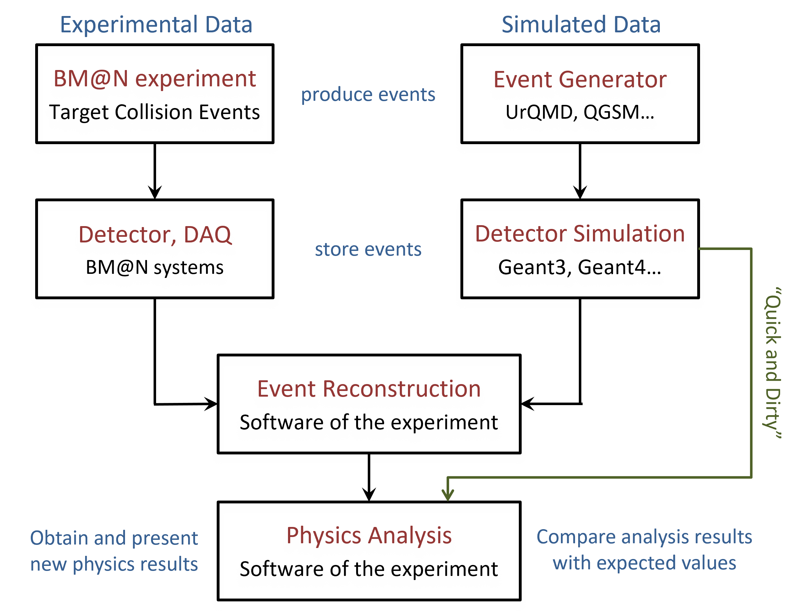
Figure 7. The chain of event processing for experimental and simulated data

To reconstruct BM@N events, the run_reco_bmn.C macro is used. The same macro processes both simulated data (the result of run_sim_bmn.C) and experimental data (the digit files of run_raw_bmn.C): the type of the input file is recognised automatically.

Function parameters of the macro run_reco_bmn.C:

Parameter	Description
TString inFileName	Input file with simulated data or with digits of experimental data. Default: $VMCWORKDIR/macro/run/bmnsim.root
TString dstFileName	Result file with reconstructed data in the DST format. Default: $VMCWORKDIR/macro/run/bmndst.root
Int_t nStartEvent	Number (starting with zero) of the first event to process. Default: 0
Int_t nEvents	Number of events to process after nStartEvent, 0 – all events of the input file. Default: 0
TString geometryTag	Tag of the setup geometry in the Geometry Database for experimental data; the empty string means the latest approved setup of the run period. For simulated data, the geometry is taken from the input file. Default: ""
enumTracking tracking	Algorithm of the inner tracking: VectorFinder, L1Tracking or CellAuto. Default: VectorFinder

Examples of the reconstruction of MC and experimental (Run 9) data:

root -b -q '$VMCWORKDIR/macro/run/run_reco_bmn.C("bmnsim.root", "bmndst.root", 0, 0)'
root -b -q '$VMCWORKDIR/macro/run/run_reco_bmn.C("bmn_run9696_ev2_p25_digi.root", "bmndst_9696_ev2_p25.root")'

The main macro lines are described below. On the first step, the macro creates the FairRunAna (run analysis) class. For simulated data, the input source is FairFileSource, the run period is taken from the metadata of the simulation file, and the geometry and the magnetic field are restored from the parameter containers of the input file. For experimental data, the input source is BmnFileSource, which defines the period and run numbers of the digit file; the geometry is loaded from the Geometry Database, and the magnetic field scale, beam and target are taken from the Unified Condition Database (UniConDa) by the run number:

FairRunAna* fRunAna = new FairRunAna();
fRunAna->SetSource(new BmnFileSource(inFileName, run_period, run_number));
// run parameters from the Unified Condition Database
UniRun* pCurrentRun = UniRun::GetRun(run_period, run_number);
fRunAna->SetSink(new FairRootFileSink(dstFileName));

The data reconstruction and physics analysis in BmnRoot are organized by a list of tasks (tasks can also be used in the simulation with the FairRunSim class). Each task participating in event processing is inherited from the base class FairTask (TTask). Three main functions of tasks can be noted. Init() function initializes the task and its variables and is executed inside the FairRunAna::Init() function. Exec(Option_t* option) function contains the main code of the task and is called by the FairRunAna::Run() function for every event. Finish() function is called at the end of the run, e.g. to write the results of the task. The scheme of task initialization and execution is presented in figure 8.

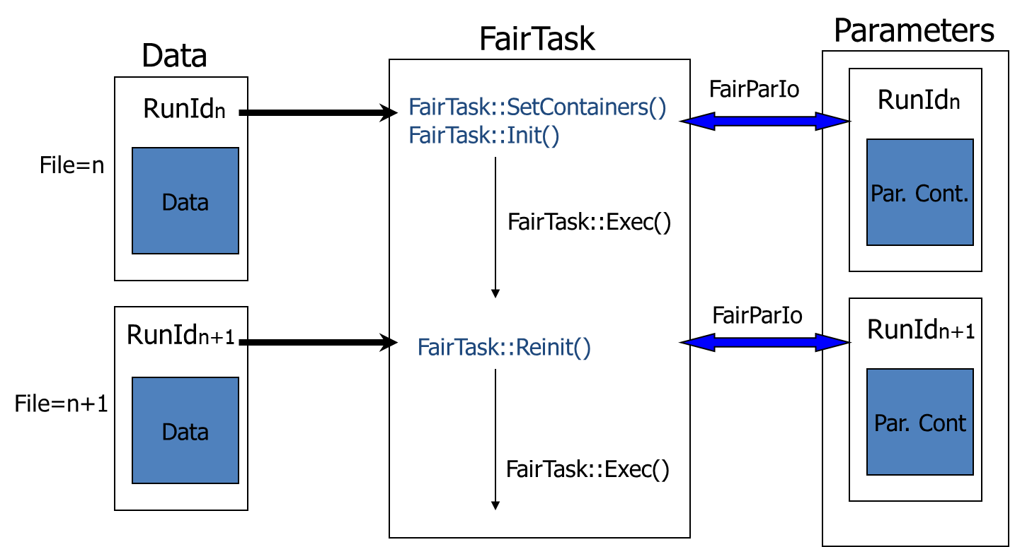
Figure 8. The scheme of task initialization and execution

The following example demonstrates task definition and adding to the task list in run_reco_bmn.C macro:

BmnGemStripHitMaker* gemHM =
    new BmnGemStripHitMaker(run_period, run_number, isExp);
fRunAna->AddTask(gemHM);

In general, a task can be added not only to the FairRunAna instance but also to another task, i.e., all tasks can be organized into a hierarchy. The detector geometry is available in all the tasks via the gGeoManager pointer: it is loaded in the main macro before the Init() functions of the tasks are called – for experimental data from the Geometry Database, and for simulated data from the FairGeoParSet container of the input file during fRunAna->Init().

The reconstruction tasks of run_reco_bmn.C for the run periods starting with Run 8 are executed in the following order:

Task (class)	Purpose
BmnFillTrigInfoDst	trigger and beam counter information
BmnSiBTHitMaker	hits in the Silicon Beam Tracker (experimental data)
BmnVSPHitMaker, BmnSiliconHitMaker, BmnGemStripHitMaker, BmnCSCHitMaker	hits and clusters of the strip detectors: VSP, Forward Silicon Detector, GEM and CSC
BmnTof1HitProducer	TOF-400 and TOF-700 hits
BmnFHCalReconstructor, BmnScWallReconstructor, BmnHodoReconstructor, BmnNdetReconstructor	forward detectors: FHCal, ScWall, hodoscope and neutron detector
BmnToCbmHitConverter	preparation of the VSP, Silicon and GEM hits for the inner tracking, including alignment corrections
BmnStsVectorFinderV9 (or L1 tracking), BmnStsMatchTracks	finding and fitting of the inner tracks, matching to MC tracks for simulated data
BmnBeamTracking	beam tracks in the SiBT (experimental data)
CbmFindPrimaryVertex, BmnKFPrimaryVertexFinder, BmnCombineVertexFinder	primary vertex finding
BmnGlobalTracking	global tracks: matching of the inner tracks with TOF-400, TOF-700 and ScWall hits
BmnMatchRecoToMC	matching of the global tracks to MC tracks (simulated data)
BmnDedx	dE/dx and charge estimate (Run 8)
CentralityClusterizer	centrality class of the event
BmnFillDstTask	event and run headers of the DST file

Figure 9 presents the main modules of the BmnRoot framework and their relationship during the reconstruction.

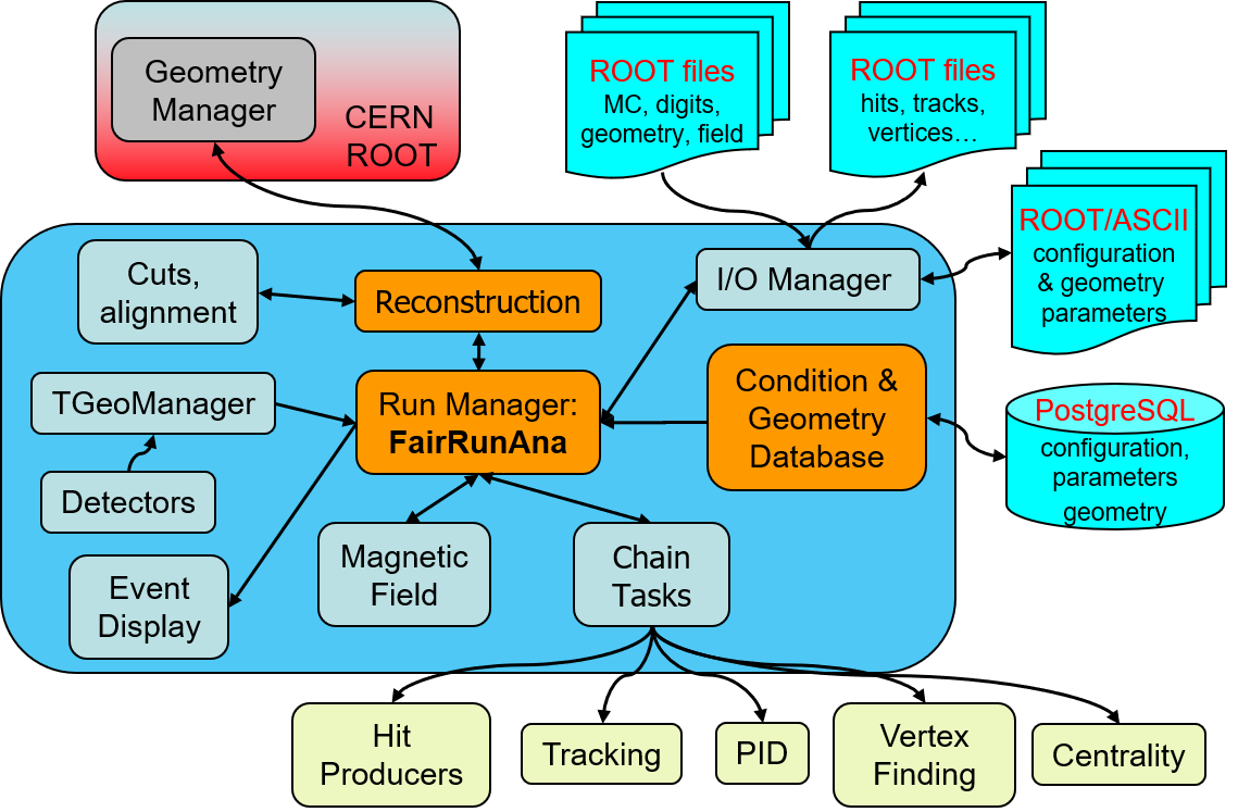
Figure 9. The scheme of the BmnRoot modules in the reconstruction

The result DST file contains reconstructed (physics and geometrical) data about particles and particle tracks of collision events registered by the BM@N facility: the event tree bmndata with the event header, trigger information, hits and clusters of the tracking detectors, inner and global tracks, primary vertices, data of the forward detectors and the event centrality, and, for simulated events, MC tracks and matching information; as well as the run header (DstRunHeader) and the geometry used in the reconstruction (FairGeoParSet). The DST format is common for simulated and experimental data and is described in detail in the separate document “BmnRoot DST Format”.

4.6 Physics analysis of reconstructed data

DST files are the input of physics analyses of the BM@N data. The recommended way is to implement every analysis as a FairRoot task and to run it with the run_ana_bmn.C macro, which is the main macro for physics analysis of simulated and experimental DST files. It sets up FairRunAna with the DST as input and executes a list of analysis tasks for every event. The macro takes care of the common steps, so that a task contains only the analysis itself:

• the input can be one DST file, a text file with a list of DST files, or a ROOT file with a TChain of DST files; all files are processed as one data set;
• the magnetic field and the run information (period, run, beam, target, energy) are taken from the first DST file (DstRunHeader), and the geometry is restored from its FairGeoParSet container;
• the Kalman filter (CbmKF) is initialised, so that the tasks can extrapolate tracks through the detector material and the magnetic field;
• the results of the tasks (histograms, trees, new branches) are written to the output file.

Function parameters of the macro run_ana_bmn.C:

Parameter	Description
TString dstFileName	Input: DST file, text file with a list of DST files, or ROOT file with a TChain of DST files. Default: $VMCWORKDIR/macro/run/bmndst.root
TString anaFileName	Result file with the analysis results. Default: $VMCWORKDIR/macro/run/bmnana.root
Int_t nStartEvent	Number (starting with zero) of the first event to process. Default: 0
Int_t nEvents	Number of events to process after nStartEvent, 0 – all events of the input file(s). Default: 10

root -b -q '$VMCWORKDIR/macro/run/run_ana_bmn.C("bmndst.root", "bmnana.root", 0, 0)'

Each analysis is a class derived from FairTask with three main methods:

• Init() – called once before the event loop: get the DST branches with FairRootManager::GetObject(), book histograms, read parameters;
• Exec() – called for every event: the objects obtained in Init() contain the data of the current event;
• Finish() – called once after the event loop: write the results to the output file.

The analysis tasks are kept in the physics library of BmnRoot. The BmnAnalysisTask class (physics/BmnAnalysisTask.h and .cxx) is a template to start from, and BmnTwoParticleDecay (physics/decay) is an example of a complete analysis task. A new task is added to physics/CMakeLists.txt and physics/PhysicsLinkDef.h; it can also be created from the NewTask template of FairRoot (Section 9.1). The example below fills the transverse momentum spectrum of the primary global tracks (for brevity, the methods are defined in the class body):

// BmnPtAnalysis: example analysis task - pt spectrum of primary global tracks
class BmnPtAnalysis : public FairTask
{
  public:
    BmnPtAnalysis() : FairTask("BmnPtAnalysis") {}
 
    InitStatus Init() override
    {
        // get the DST branches from the input of FairRunAna
        FairRootManager* ioman = FairRootManager::Instance();
        fGlobalTracks = (TClonesArray*)ioman->GetObject("BmnGlobalTrack");
        fInnerTracks = (TClonesArray*)ioman->GetObject("StsVector");
        fVertex = (CbmVertex*)ioman->GetObject("MpdVertex.");
        if (!fGlobalTracks || !fInnerTracks || !fVertex) {
            LOG(error) << "BmnPtAnalysis::Init(): DST branches not found";
            return kERROR;
        }
        fHistPt = new TH1D("hPt", "p_{T} of primary tracks;p_{T}, GeV/c;N",
                           100, 0., 3.);
        return kSUCCESS;
    }
 
    void Exec(Option_t* /*option*/) override
    {
        if (fVertex->GetNTracks() < 2)
            return;
        for (Int_t i = 0; i < fGlobalTracks->GetEntriesFast(); i++) {
            auto* track = (BmnGlobalTrack*)fGlobalTracks->UncheckedAt(i);
            Int_t iInner = track->GetGemTrackIndex();
            auto* inner = (CbmStsTrack*)fInnerTracks->UncheckedAt(iInner);
            if (!inner->FromVertex())   // not used in the primary vertex fit
                continue;
            fHistPt->Fill(track->GetPt());
        }
    }
 
    void Finish() override
    {
        // write the results to the output file of run_ana_bmn.C
        FairRootManager::Instance()->GetSink()->WriteObject(fHistPt, "hPt");
    }
 
  private:
    TClonesArray* fGlobalTracks = nullptr;
    TClonesArray* fInnerTracks = nullptr;
    CbmVertex* fVertex = nullptr;
    TH1D* fHistPt = nullptr;
 
    ClassDefOverride(BmnPtAnalysis, 1);
};

The task is created in the “Analysis Tasks” block of run_ana_bmn.C:

CbmKF* kalman_filter = new CbmKF();
fRunAna->AddTask(kalman_filter);
 
BmnPtAnalysis* pt_analysis = new BmnPtAnalysis();
fRunAna->AddTask(pt_analysis);

Several analyses can run in one pass over the data: add one task for each of them. The tasks are executed in the order in which they are added, so a task can use objects that a previous task registered with FairRootManager::Register().

For quick checks, the DST tree can also be read directly in a ROOT macro (see, for example, macro/howTo/readDst.C) or with TTree::Draw, where the names of the data members can be used in the expressions:

TFile* f = TFile::Open("bmndst.root");
TTree* t = (TTree*)f->Get("bmndata");
t->Draw("MpdVertex.fZ", "MpdVertex.fNTracks > 1");   // vertex z
// beta of the tracks matched to TOF-400 hits
t->Draw("BmnGlobalTrack.fBeta400", "BmnGlobalTrack.fTof1Hit >= 0");

The full description of the DST content – branches, classes and their fields, links between the objects, differences between simulated and experimental DST files – and examples of the physics analysis are given in the “BmnRoot DST Format” document.

5. Event Display of the BM@N Experiment

5.1 ROOT Geometry Package

The ROOT geometry package is a tool to build, browse and visualize detector geometries. It is independent from any tracking Monte Carlo engine, though it has been designed to optimize particle transport in correlation with simulation packages as Geant3, Geant4 and Fluka.

The building blocks of any geometry are the volumes that may contain other volumes. The biggest one, called the “cave”, contains all other volumes and provides the master reference system (MARS) in which the others are positioned. Each volume needs to be associated with a medium that can be a mixture of different materials (whose weights are the relative densities). An example of creating of the simplest setup having a single empty box in the ROOT environment (CLING) is presented below.

root[] gSystem->Load("libGeom"); // load the ROOT geometry library
root[] TGeoManager* mng = new TGeoManager("cave", "the simplest geometry");
root[] TGeoMaterial* mat = new TGeoMaterial("Vacuum", 0, 0, 0);
root[] TGeoMedium* med = new TGeoMedium("Vacuum", 1, mat);
root[] TGeoVolume* top = gGeoManager->MakeBox("Top", med, 10., 10., 10.);
root[] gGeoManager->SetTopVolume(top);
Info in <TGeoManager::SetTopVolume>: Top volume is Top. Master volume is Top
root[] gGeoManager->CloseGeometry();
Info in <TGeoManager::CheckGeometry>: Fixing runtime shapes...
Info in <TGeoManager::CheckGeometry>: ...Nothing to fix
Info in <TGeoManager::CloseGeometry>: Counting nodes...
Info in <TGeoManager::Voxelize>: Voxelizing...
Info in <TGeoManager::CloseGeometry>: Building cache...
Info in <TGeoManager::BuildCache>: --- Maximum geometry depth set to 100
Info in <TGeoManager::CloseGeometry>: 1 nodes/ 1 volume UIDs in title
Info in <TGeoManager::CloseGeometry>: --- modeler ready ---
root[] top->SetLineColor(kMagenta);
root[] mng->SetTopVisible(); // the TOP is generally invisible
root[] top->Draw();
--- Drawing        1 nodes with 3 visible levels
<TCanvas::MakeDefCanvas>: created default TCanvas with name c1

The last command pops up a new window displaying a canvas with the magenta cube. It is possible to move, rotate and zoom the camera interactively by clicking and dragging the mouse.

Complex geometries can be built in a hierarchical way, through the concept of containment: one has to define and position some volumes inside other ones. Positioning is done with spatial transformations with respect to the "mother reference system" (i.e., the system defined by the containing volume). Complex volumes are built using basic or primitive shapes, already defined by ROOT (e.g., box, tube, cone, etc.), through operations like join, subtract or intersect. Finally, a given volume can be positioned several times in the geometry or it can be divided accordingly to user-defined patterns, automatically defining new contained volumes.

Once a geometry has been created, it can be saved into a ROOT file or as C++ macro with the Export(...) method of TGeoManager. Loading the geometry is done with its Import(...) method. In addition, individual volumes can also be saved into a ROOT file. Finally, ROOT provides a graphical user interface to edit or build geometry. The editor can be opened with the Edit(...) method of TGeoManager.

The possibility to visualize 3D objects is very important: in ROOT, the rendering engine is provided by the OpenGL library that provides advanced visualization features and real-time animations. Event display applications are an important application of 3D visualization.

5.2 Event Display of the Experiment

One of the commonly solved problems in modern high-energy physics experiments on particle collisions is the visual representation of the events during the experiment run. Event display system can be used at the design stage of the detectors for:

• model and reconstruction algorithm checking and debugging by developers;
• analysis of algorithms for event data processing by experts;
• visualization of data reconstruction and physics analysis for better understanding of the detectors and collision event structure by users;
• demonstration and presentation of results of an experiment.

In addition, event display can be used at the run stage for online visual monitoring of selected events during the experiment run with the aim of visual control and debugging of current events. Visual monitoring of physical processes and data is very important, for example, for visual estimation of the multiplicity of current events, which depends on the impact parameter of the collision.

The event display package is a part of the BmnRoot environment. The event visualization uses data of the experiment as follows (figure 10). The data (types of particles produced, their momenta and other kinematic parameters) obtained by event generators such as UrQMD and QGSM are passed to simulation macro transferring the particles through the detectors by particle transport packages (Geant). The setup geometry loaded from the Geometry Database is presented by a hierarchy of the ROOT geometric shapes, transformation matrices and other graphics information, which is stored in the result ROOT file. After the simulation has been completed, the resulting file contains both the Monte Carlo data and the BM@N geometry.

The next step is the reconstruction of particle data, tracks and other parameters that are written to DST file. The reconstruction algorithms restore the information about the particle trajectory and identity from the information contained in the simulated (or raw) detector data. The MC and DST data are stored in ROOT files in a hierarchical tree view.

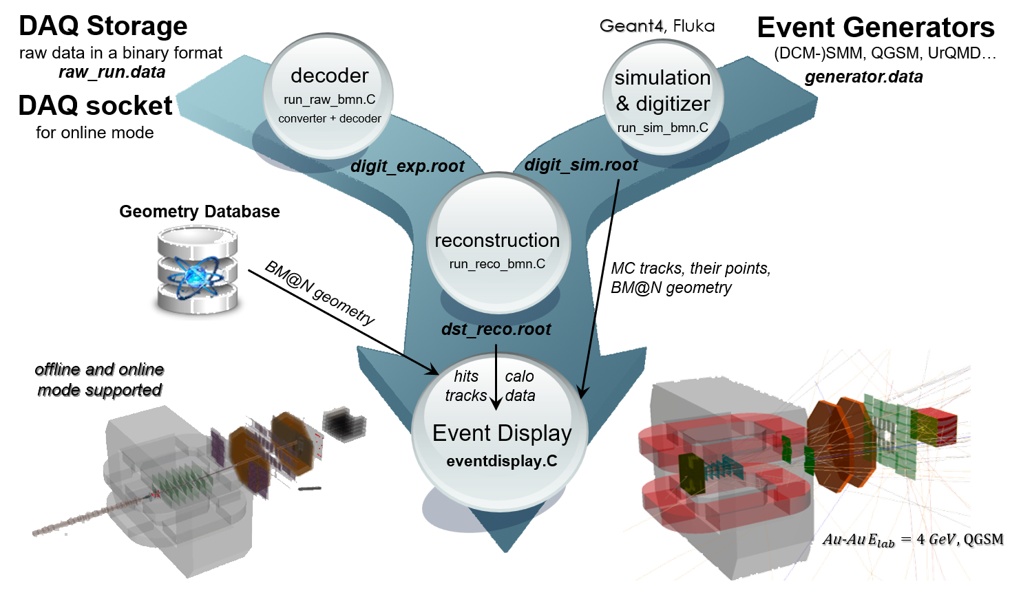
Figure 10. Input data for BM@N event display

For graphical representation of the simulated events, the developed eventdisplay.C macro uses both the file with the simulated data together with the BM@N geometry and the DST file with the reconstructed data. Experimental data are also supported: in this case, the reconstructed information is taken from the DST file in the same way as for simulated events, and the BM@N setup geometry is loaded from the Geometry Database. In addition, the event display has the online mode to visualize events during the experiment runs. The event display is integrated with the BmnRoot software to combine different stages of the event processing with a graphical representation of these events with the aim to evaluate and check the correctness of reconstruction and physics analysis algorithms. In addition, it enables one to take into account adding the subdetectors to the facility structure and changing the current configuration of the BM@N setup.

To display detector geometry and events of the BM@N experiment the high-level graphics package EVE is used, which provides graphical representation and management of visualization objects for high energy physics. The package uses ROOT GUI environment and OpenGL library to display three-dimensional objects and its two-dimensional projections. The EVE classes developed primarily for the creation, management of event objects such as raw data, hits, clusters, points (TEvePointSet), and particle tracks (TEveTrack), allow selecting and highlighting different elements, configuring its parameters.

To visualize events of the BM@N experiment new classes have been developed for the management of different physical objects and their graphical representation, e.g., MC points (MpdMCPointDraw class), simulated particle trajectories (MpdMCTracks), reconstructed hits (MpdHitPointSetDraw) and tracks (BmnTrackDrawH, BmnGlobalTrackDraw), calorimeter towers (BmnCaloTowerDraw). These classes are located in ‘eventdisplay’ directory. MpdEventManager main class (inherits from TEveEventManager) has been developed to perform the following functions: read events directly from ROOT tree, select events for display, apply cuts to events, event navigation (next event, previous event and go to event number), read and display the detector geometry.

The event display macro (macro/eventdisplay/eventdisplay.C) provides users with control and graphical representation of detector geometry, MC tracks and their points, as well as reconstructed hits, tracks, energy deposited in calorimeter towers. It reads detectors’ geometry, simulated and reconstructed event data from the ROOT files and displays the objects by the EVE package. All necessary options for graphical representation of the physical objects are included in the macro, set by default, and can be changed.

Function parameters of the macro eventdisplay.C:

Parameter	Description
TString simFile	Input file with MC data and detector geometry for visualization of simulated events. Default: $VMCWORKDIR/macro/run/bmnsim.root
TString recoFile	Input file with reconstructed data (DST) of simulated or experimental events. Default: $VMCWORKDIR/macro/run/bmndst.root
TString endpoint	Address of the ZeroMQ publisher socket, e.g. tcp://localhost:5557; if it is not empty, the event display is started in the online mode. Default: "" (offline mode)

root '$VMCWORKDIR/macro/eventdisplay/eventdisplay.C("bmnsim.root", "bmndst.root")'

In the offline mode, the type of data is recognised by the reconstructed file. For simulated data, the simulation file is opened as the input source with the DST file added as a friend, and the detector geometry is read from the simulation file. The following tasks are added to the event manager to display the objects:

• MpdMCPointDraw – MC points of the subdetectors (e.g. SiliconPoint, StsPoint, CSCPoint, TOF400Point branches);
• MpdMCTracks – simulated particle trajectories stored in the GeoTracks branch (the simulation has to be run with saveGeoInfo = kTRUE);
• MpdHitPointSetDraw – reconstructed hits of the detectors (e.g. BmnSiliconHit, BmnGemStripHit, BmnCSCHit, BmnTof400Hit, StsHit);
• BmnCaloTowerDraw – calorimeter modules (towers) with energy depositions;
• BmnTrackDrawH – tracks drawn by their hits, e.g. inner tracks (StsVector) and beam tracks (BmnBeamTrack);
• BmnGlobalTrackDraw – reconstructed global tracks.

For experimental data, the DST file is the input source, and the geometry of the BM@N setup is loaded from the Geometry Database – the latest approved setup of the defined run period (Section 6.2). The same tasks are used to draw the reconstructed objects. In the online mode, the event display receives events from the online reconstruction via ZeroMQ and continuously shows them.

The event display shows the BM@N geometry and events in different projections and views, and has a multiview mode. A user can select the tab with a convenient graphical representation, set light sources, configure physical objects’ parameters, for example, specify a desired color of the object or a background color. The event display offers full interactivity, supporting on-line rotations and picking of objects. Three methods of geometry coloring have been implemented in the visualization system: default by ROOT, hierarchical and pre-selected for detectors. In the case of hierarchical coloring, a user can choose colors for the different levels of the BM@N geometry tree. If the pre-selected mode is chosen, a color can be set for each subdetector of the facility. The coloring and other settings of the event display are defined in the config/eventdisplay.json file, and examples of the coloring schemes are located in the macro/eventdisplay/examples directory. Figure 11 presents visualization of the BM@N detector in the multiview mode: 3D view together with XY and XZ projections.

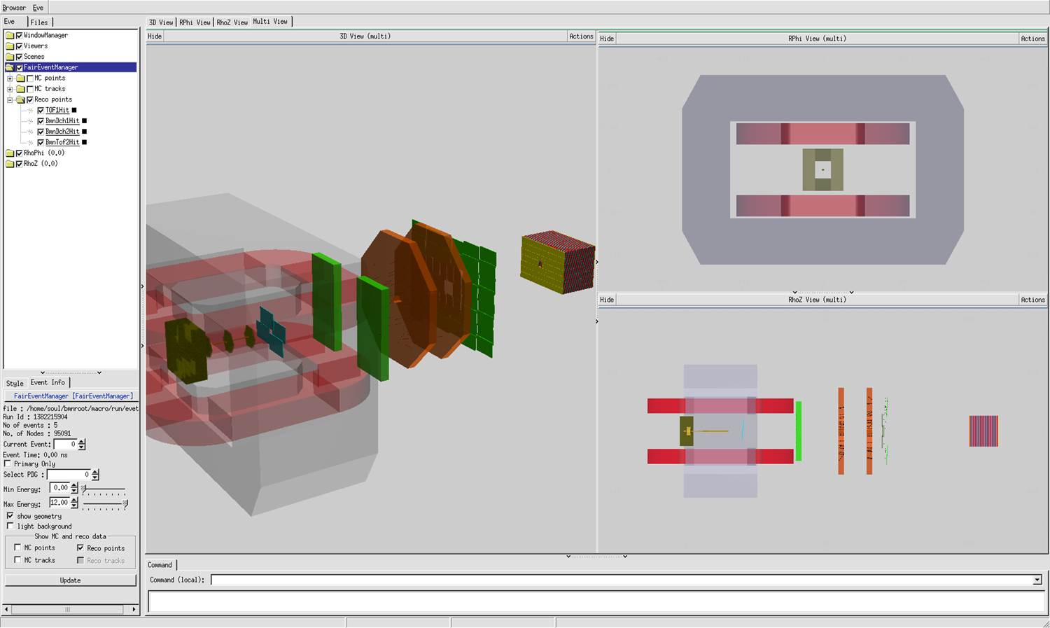
Figure 11. The views and projections of the BM@N facility in the event display

Figure 12 presents MC tracks (simulated by UrQMD generator) of the central event in collisions of bismuth ion beam with a bismuth target at the energy 4 GeV per nucleon. Tracks of different particles are highlighted in different colors. The EVE package provides a browser (on the left side of the window) to all the displayed objects. The object browser includes both geometry and event information presented in a hierarchical tree. Users can select in the tree individually which objects to draw, change object colors and set other visualization settings. In addition, the event display provides quick access to the following settings of event representation:

• selecting an event number displayed on the screen;
• showing all or only primary particles, particles with given PDG codes;
• setting energy range of particles to be displayed;
• changing the background of BM@N views and projections;
• choosing objects to be presented on the screen: MC tracks and their points, reconstructed hits and particle tracks.

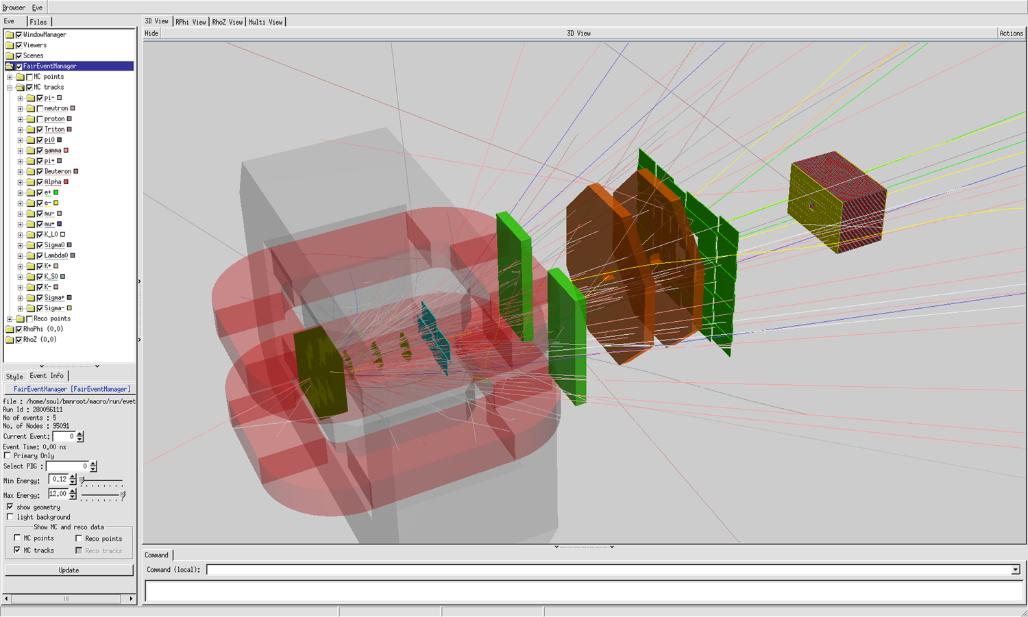
Figure 12. BM@N event visualization of MC tracks in Bi – Bi collision at 4 GeV/nucleon

As a result, the event display system allows one to compare the simulated and reconstructed data visually to verify the correctness of developed algorithms. In order to clearly compare hits and particle tracks the display option has been implemented to hide the entire BM@N geometry on the screen. Additionally, the option for high transparency of detector geometry has also been developed (figure 13). It sets the different transparency coefficients appropriated for different BM@N subdetectors.

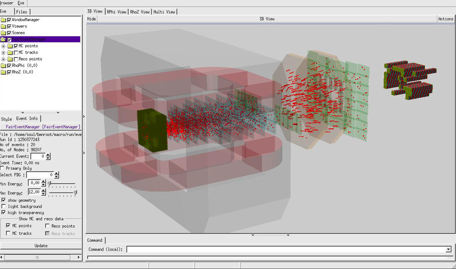
Figure 13. Event display for Bi – Bi collisions in the high transparency mode

6. Information Systems of the BM@N Experiment

To store, manage and provide the information required for the processing and analysis of the BM@N data, a complex of information systems has been developed for the BM@N experiment. Each system is based on a database and provides a Web service for the collaboration members and application programming interfaces (REST API and/or C++ interface) for other software systems of the experiment. The stored data are backed up automatically to ensure that the data of the experiment will not be lost due to software or hardware failures. The C++ interfaces of the information systems are located in the database directory of BmnRoot, each in its own subdirectory with examples and the settings header file, which defines the connection parameters, including the login and password used by the interface (e.g. uni_db_settings.h), whereas the JINR account (SSO) of the user is employed for the authorization in the Web services. A request for the rights to view and edit the information of the systems can be submitted on the official site of the experiment (bmn.jinr.int/registration). The information systems of the BM@N experiment that have an interface in BmnRoot are listed in the table below.

Information system	Purpose	Web service	Interface in BmnRoot
Unified Condition Database (UniConDa)	parameters of the runs, detectors and simulation files used in the data processing	bmn-uniconda.jinr.int	database/uni_db (Section 6.1)
Geometry Database	geometry setups of the experiment	bmn-geometry.jinr.int	database/geo_db (Section 6.2)
Electronic Logbook (e-Log)	shift records on the runs and operation conditions of the systems	bmn-elog.jinr.int	database/elog_db (Section 6.3)
Event Metadata System (EMS)	catalogue of the event metadata for the selection of events	bmn-event.jinr.int	database/event_db (Section 6.4)
Data Management System (DMS)	file catalogue of the experiment data on the distributed storages	–	database/file_db (Section 6.5)
Slow Control Viewer (SC Viewer)	viewing the hardware parameters of the detectors and systems recorded by the Slow Control System	bmn-tango.jinr.int	database/tango (Section 6.6)

6.1 Unified Condition Database

6.1.1 Purpose of the Unified Condition Database

Today the use of databases is a prerequisite for qualitative management and unified access to the data of modern high-energy physics experiments. The Unified Condition Database (UniConDa) is designed as comprehensive relational data storage for offline data analysis in the high-energy physics experiments. It provides unified access and data management for all collaboration members, correct multi-user data processing, ensuring the actuality of the information being accessed (run parameters, detector geometries and positions, technical and calibration data, etc.), data consistency and integrity, excluding the multiple duplication and use of outdated data.

The parameter data being stored in the Unified Condition Database can be classified into 4 groups:

1. Configuration data are concerned with the detector running mode, i.e., programmable parameters for frontends electronics.
2. Calibration data describe the calibration and the alignment of the different subdetectors. Usually, quantities are evaluated by running dedicated offline algorithms.
3. Parameter data present the state of detector subsystems. They include a variety of detector settings including the geometry and material definitions.
4. Algorithm data are used to control the way algorithms operate. They include, for example, cuts for selection and production paths of files.

The Unified Condition Database is developed for the fixed target experiment BM@N of the NICA project. The runtime parameter manager of FairRoot initializes parameters from ROOT or ASCII files, but it cannot work with a database system, therefore the C++ interface of the database has been developed for BmnRoot (Section 6.1.2).

Entity-relationship diagram of the Unified Condition Database is shown in figure 14. The database includes the following groups of tables: metadata of the runs and raw data files (run periods, runs, raw files), the parameter warehouse (detectors, parameter types, parameters and parameter values of the detectors for the ranges of runs), and the metadata of the simulation files. The detailed description of the database tables and their attributes is given in the Unified Database User Guide (database/uni_db/docs directory).

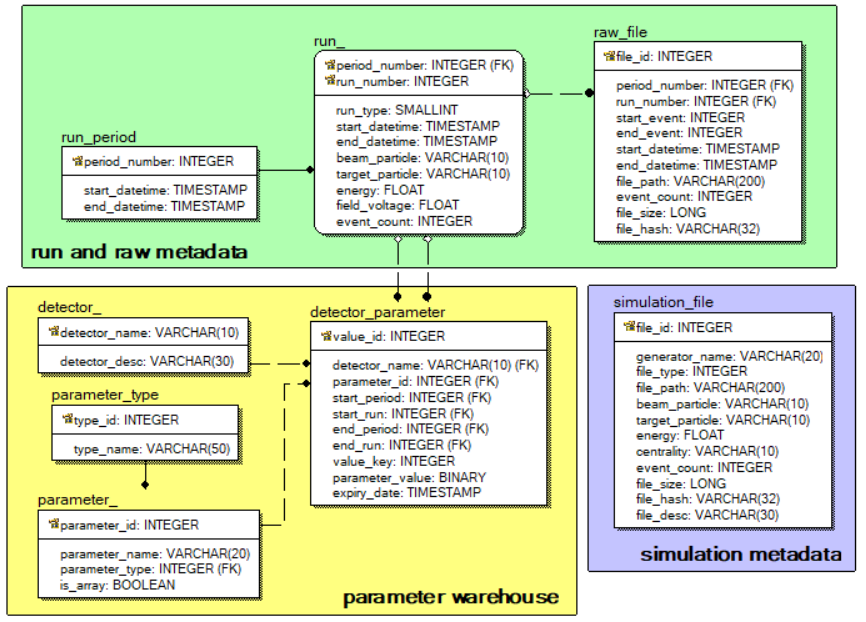
Figure 14. ER-diagram of the Unified Condition Database

The Unified Condition Database implemented on the PostgreSQL DBMS (database management system) provides user access to the actual experiment parameters. Each value of a detector parameter is stored with its validity period – the range of runs, for which the value is valid. In addition, all previous values of the parameters are kept: when a parameter value is changed, the old value is not deleted, but marked by its expiry date (the expiry_date attribute), so that the data can be processed with the parameter values used before (the usage_time argument of the UniDetectorParameter::GetDetectorParameter function).

By default, BmnRoot users have a read-only access to the Unified Condition Database. To get other privileges, set your login and password in the UNI_DB_USERNAME and UNI_DB_PASSWORD constants of the database/uni_db/uni_db_settings.h file and rebuild BmnRoot. To test connection to the database, you can run the test_db.C macro: “root -b -q $VMCWORKDIR/database/uni_db/macros/test_db.C”.

The common communications scheme of the Unified Condition Database is presented in figure 15.

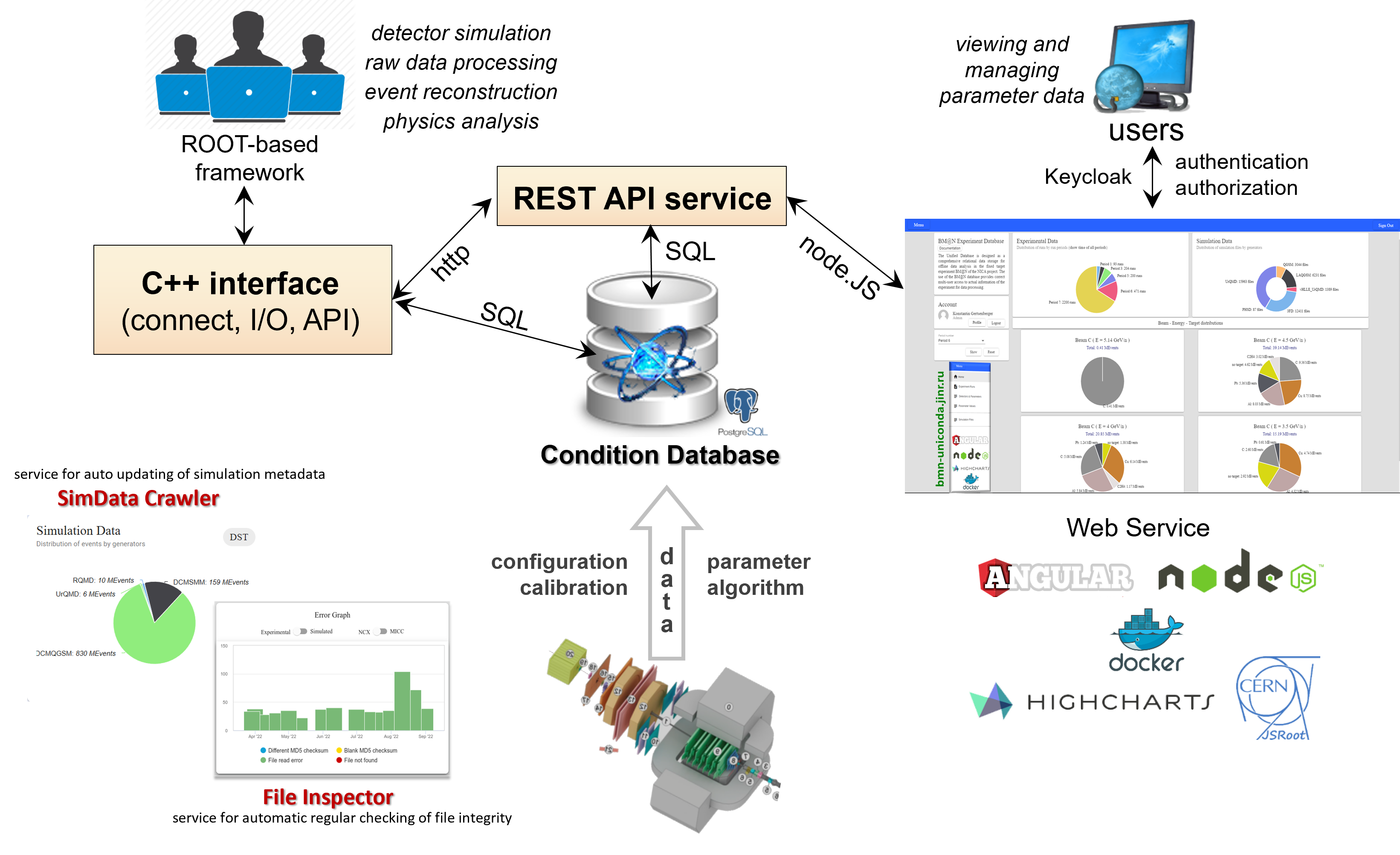
Figure 15. The common communications scheme of the Unified Condition Database

The BmnRoot environment uses the C++ database interface to get information for raw data processing, simulation, event reconstruction and physics analysis tasks. The Web interface of the Unified Condition Database (bmn-uniconda.jinr.int) allows users to browse and search the information on the run periods, runs, raw data files, detector parameters and simulation files.

6.1.2 C++ Interface of the Unified Condition Database

To process data of the experiment, the C++ database interface has been implemented as a set of C++ class wrappers for all database tables with many specific functions. It allows one to work with the data of the Unified Condition Database without any SQL statements. The interface is located in the database/uni_db directory, and its classes are described in the Unified Database User Guide and Reference Manual (database/uni_db/docs). These classes allow managing information about run periods, runs, raw files, detectors, parameters and their values, and generated simulation files:

• UniRunPeriod – run periods (sessions) of the BM@N experiment;
• UniRun – run parameters (number, start and end time, beam, target, energy, magnetic field voltage, event count, etc.);
• UniRawFile – information on raw data files of the runs;
• UniDetector – detectors of the BM@N experiment (detector dictionary);
• UniParameter – common information about the detector parameters stored in the database (parameter dictionary);
• UniDetectorParameter – values of the detector parameters for the experiment runs with their validity periods (ranges of runs);
• UniSimulationFile – information on simulation files produced by different event generators, such as UrQMD and DCM-SMM.

The classes have main static functions to manage corresponding whole objects: Create, Delete, Get, Search, PrintAll, and non-static functions to work with their attributes: Getters and Setters functions, Print. For example, the parameters of a run can be obtained as follows:

UniRun* pRun = UniRun::GetRun(9, 9696);   // period 9, run 9696
if (pRun != nullptr) {
    cout << pRun->GetBeamParticle() << " + "
         << pRun->GetTargetParticle() << endl;
    delete pRun;
}

Some additional classes of the C++ database interface have been developed: UniConnection class serves to open and close database connections, UniSearchCondition class forms criteria for the selection of runs, files and detector parameters, and UniValue classes present parameter values of different types. In addition, the interface includes numerous examples of using the C++ interface (database/uni_db/examples, e.g. get_parameter_value.C, selecting_runs.C) and console utilities (show_experiment_files, show_simulation_files) to search for experimental and simulation files by their parameters.

6.2 Geometry Database

6.2.1 Purpose of the Geometry Database

The geometry of the BM@N setup changes from one Run to another: detectors are added, removed, replaced by new versions or moved to new positions, and the detector models are refined. When the setup geometry is assembled from a set of geometry files by a macro, it is difficult to guarantee that the same geometry is used in the simulation, reconstruction and analysis of different data sets. To solve the problem, the Geometry Information System has been developed. Its main component, the Geometry Database, stores, processes and manages the information on geometry models of the detectors and complete setups of the experiment, so that a setup is uniquely identified by its tag.

The main objects of the Geometry Database are the following:

• module – a detector or a passive element of the setup (cave, magnet, target, beam pipe, SiBT, VSP, Silicon, GEM, CSC, TOF-400, TOF-700, FHCal, ScWall, Hodo, Ndet, etc.) together with the BmnRoot class implementing it, e.g. BmnSilicon, CbmSts (GEM), BmnTOF1, FairMagnet;
• geometry file – a version of the module geometry in ROOT (.root) or ASCII (.geo) format;
• setup module – a geometry module placed in a setup: its position (translation and rotation), tag and, if required, the parameter file of the detector;
• setup – the complete geometry of the BM@N facility, defined by a list of the setup modules, the media (materials) file and the magnetic field (e.g. a field map with the Hall voltage value at which it is measured); the setup also includes a ROOT file with the full geometry of the facility.

Each setup is identified by a unique tag, which includes the run period, e.g. run9_26.09.0. A setup can be approved by the persons responsible for the geometry: the approved setups are the recommended ones for the data processing. The tags of the approved setups are formed as run<N>_dev_YY.MM.DD for the development versions, where YY.MM.DD is the creation date of the setup, and as run<N>_YY.MM.P for the production versions, where YY.MM.P is the tag of the BmnRoot release (P is the patch number of the release starting from 0). N is the number of the run period, e.g. run9_dev_26.05.23 and run9_26.09.0.

The central Geometry Database is accessible via the Geometry Web Service of the experiment (https://bmn-geometry.jinr.int), which allows browsing the setups with their modules and downloading the replica of the database. Users with the rights to edit the geometries of certain detectors can upload and edit the geometry versions of these detectors via the Geometry Web Service, and the lead developers can also compose new setups from the detector geometries and approve them. BmnRoot works with a local replica of the database: the SQLite file local.db together with the storage directory containing the geometry, media and field map files, both located in the database/geo_db directory.

6.2.2 Using the Geometry Database in BmnRoot

The interface of the Geometry Database is located in the database/geo_db directory of BmnRoot. The location of the local replica is set by the DBL_FILE_PATH environment variable (path to the directory of the local.db file), which is exported by the config.sh script of the BmnRoot build. If a requested geometry setup is absent in the local replica or a newer version of a not approved setup exists, the setup is downloaded from the central database automatically. If the directory of the replica is read-only (e.g. on CVMFS), the replica is installed to a writable directory: $DBL_CACHE_PATH, if it is set, $TMPDIR or /tmp/<user>. The list of setups in the local replica is printed by the macro:

root -b -q $VMCWORKDIR/database/geo_db/macros/getSetupList.C

The setups are loaded by the GeoSetup class, which has the following main methods:

• LoadSetupToFairRunSim(setup_tag, localSettings) – loads the modules of the setup with their positions, media and the magnetic field to the FairRunSim instance for the simulation; the optional localSettings argument is a path to an XML file with a local customization of the setup (Section 6.2.3);
• LoadSetupToGeoManager(setup_tag) – loads the full geometry of the setup as the gGeoManager instance for the reconstruction and analysis;
• GetLastApprovedSetupTag(prefix) – returns the tag of the latest approved setup, which starts with the given prefix, e.g. "run9";
• GetMagneticField(scale) – returns the magnetic field of the current setup (an instance of a class derived from FairField) with the given scale of the field map (zero value turns the field off);
• GetParameterFile(detector_name) – returns the path to the parameter file of the given detector of the current setup;
• GetMaterialFile() – returns the media file of the current setup.

The Geometry Database is used at all stages of the BM@N data processing:

• run_sim_bmn.C loads the setup for the simulation by the geometryTag parameter: the default value "run9:" (a tag prefix followed by ‘:’) means the latest approved setup of Run 9; the tag of the setup is saved in the description of the FairGeoParSet container of the result file;
• run_reco_bmn.C uses the geometry stored in the simulation file for simulated data, whereas for experimental data it loads the full setup geometry by the geometryTag parameter, by default – the latest approved setup of the run period of the input file; the tag is also written to the FairGeoParSet container of the DST file;
• run_ana_bmn.C takes the geometry from the input DST file;
• eventdisplay.C reads the geometry from the simulation file for simulated data, whereas for experimental data it loads the latest approved setup of the run period, which is defined by the input DST file.

Example of loading a setup geometry in a stand-alone ROOT macro:

GeoSetup gSetup;
string tag = gSetup.GetLastApprovedSetupTag("run9");   // e.g. run9_26.09.0
if (gSetup.LoadSetupToGeoManager(tag) != 0)
    cout << "ERROR: the geometry was not loaded" << endl;
gGeoManager->GetTopVolume()->Draw("ogl");

6.2.3 Local customization of the setup geometry

In some cases, it is necessary to simulate a setup, which differs from the one stored in the Geometry Database: to test a new version of a detector geometry before uploading it to the database, to study the effect of a detector shift or of a missing detector, to add a new detector prototype, etc. For such tasks, a local customization of a setup is described in an XML file, which is applied to the setup from the database during its loading for the simulation without changing the Geometry Database itself.

To apply the customization, the path to the XML file is appended to the geometry tag of run_sim_bmn.C after the ‘;’ separator, environment variables in the path are expanded:

root -b -q '$VMCWORKDIR/macro/run/run_sim_bmn.C("", "bmnsim.root", 0, 100, BOX, "run9:;$VMCWORKDIR/my_setup.xml")'

The root element of the XML file is <setup>. It can contain child elements of two types: <editSetupModule> to change or disable a module of the setup, and <addSetupModule> to add a new module to the setup. Attributes of the <editSetupModule> element:

Attribute	Description
tag	Tag of the setup module to be customized (case-insensitive), required. The tags of the modules are printed in the log of the simulation macro (“Loading module with tag=...”) and are shown on the Geometry Web Service.
enable	"false" disables (removes) the module from the setup, "true" – the module is used with the changes set by the other attributes. Default: "true"
file_path	Path to a ROOT file with a new geometry of the module to be used instead of the database one. Default: the geometry file from the database
moveX, moveY, moveZ	Shifts of the module along the X, Y and Z axes in cm relative to its position in the setup. Default: 0

Attributes of the <addSetupModule> element:

Attribute	Description
class_name	Name of the class implementing the module in the simulation, e.g. BmnHgnd, BmnFD, FairMagnet; required.
args	Name of the module passed as the first argument to the class constructor. The name is chosen by the user, preferably unique in the setup and, by convention, in upper case like the names of the database modules (SILICON, GEM, TOF400, NDET, etc.), e.g. "HGND", "MAGNET".
active	"true" for a detector with sensitive volumes producing MC points, "false" for a passive module. Default: "true"
file_path	Path to the geometry file of the new module; required.

Example of the XML file, which disables the FHCal module, replaces the geometry of the neutron detector by a local file and adds the HGND detector to the setup:

<setup>
  <editSetupModule tag="FHCal_geo_period9_v2.root" enable="false"/>
  <editSetupModule tag="Ndet_geo_period9_v2"
                   file_path="$VMCWORKDIR/my_geometry/ND_new_run9.root"/>
  <addSetupModule class_name="BmnHgnd" active="true" args="HGND"
                  file_path="$VMCWORKDIR/my_geometry/HGND_run10.root"/>
</setup>

The next example shifts a module (e.g. a tracking detector) by 0.5 cm along the X axis and by 1 cm along the Z axis to estimate the effect of such misalignment on the reconstruction:

<setup>
  <editSetupModule tag="TAG_OF_THE_MODULE" moveX="0.5" moveZ="1.0"/>
</setup>

Please, take into account the following features of the local customization:

• the customization is applied only in the simulation; the geometry with all the changes is stored in the simulation file, so the reconstruction and analysis of these simulated data use the customized geometry automatically, and the FairGeoParSet container keeps the geometry tag of the setup with the path to the XML file appended to the tag after the ‘;’ separator;
• experimental data are always reconstructed with a setup geometry from the Geometry Database: corrections of the real setup, e.g. new detector positions obtained by the alignment, have to be uploaded to the Geometry Database as a new setup instead of using the XML file;
• only translations are supported: the shifts are added to the module position in the setup, the rotation of a module cannot be changed by the XML file now; the shifts are applied to the modules defined by ROOT files, not to the cave and modules in the ASCII (.geo) format;
• a new geometry file set by file_path should be prepared in the same way as the database geometry file of the module (e.g. by the corresponding macro of the macro/geometry directory) and keep the names of the sensitive volumes, if they are used by the detector classes and digitizers;
• the simulation output reports the disabled modules (“Disable module with tag=... use local settings”) and the added detectors (“Added external detector: ...”), which helps to check the customization.

6.3 Electronic Logbook

The Electronic Logbook Platform (e-Log) replaces paper journals of the shift crew. During the experiment sessions, the shift crew records information on the runs, operation conditions of the detector systems, occurred events and problems, as well as on the taken actions. A record contains the record time and type, the shift leader name, the period and run numbers, the trigger, the status of the DAQ and of the detector systems, the beam and its energy, the target and its thickness, the magnetic field, comments and attached files. The logbook information is used in the raw data processing, reconstruction and physics analysis of the events, e.g. to select the runs with the necessary conditions.

The Web service of the e-Log (bmn-elog.jinr.int) allows users, depending on their role, to view, add and change records, attach files, as well as to sort, filter and search for records by specified criteria. In addition, collaboration members can subscribe to email notifications on new records of selected types (e.g. “new run” or “problem report”) in their personal account.

The C++ interface of the e-Log (database/elog_db directory) is implemented as a set of class wrappers for the logbook tables: ElogRecord (main records of the logbook), ElogPerson (dictionary of the persons), ElogType (dictionary of the record types), ElogTrigger (dictionary of the triggers), ElogBeam (dictionary of the beams), ElogTarget (dictionary of the targets), ElogAttachment and others. Their static functions create, get and search for records, e.g. ElogRecord::GetRecords(period, run) returns the records of the given run, and the criteria of the search are set by ElogSearchCondition objects. In BmnRoot, the interface is used, for example, by the Online Histogramming System to find reference runs with similar conditions, by the decoder and by the tasks of the trigger efficiency and QA to get the trigger of the runs. The login and password of the interface are set in the elog_db_settings.h file, and the examples of using the C++ interface are located in the database/elog_db/examples directory. Example of selecting the e-Log records of Run 8 with the CsI target:

TObjArray conds;
conds.Add(new ElogSearchCondition(ElogSearchCondition::columnPeriodNumber,
                                  ElogSearchCondition::conditionEqual, 8));
conds.Add(new ElogSearchCondition(ElogSearchCondition::columnTargetParticle,
                                  ElogSearchCondition::conditionEqual,
                                  TString("CsI")));
TObjArray* records = ElogRecord::Search(conds);
for (int i = 0; i < records->GetEntriesFast(); i++) {
    ElogRecord* record = (ElogRecord*)records->At(i);
    cout << record->GetRecordDate().AsSQLString() << endl;
}
conds.Delete();
delete records;

6.4 Event Metadata System

The Event Metadata System (EMS) is the event catalogue of the experiment, which allows collaboration members to quickly search for the physics events required for an analysis by given criteria without reading all the data files. The Event Catalogue of the EMS stores the metadata of the reconstructed events: the storage and the path of the file containing the event, the event number in the file, the version of the software used for the processing, the period and run numbers, and the number of tracks in the event. The run parameters, such as the beam particle and energy, are taken from the Unified Condition Database to preselect the runs matching the criteria of a request. The catalogue is filled with events collected in conducted runs.

The Web interface of the EMS (bmn-event.jinr.int) is convenient to check the available events: a user sets the criteria, e.g. the period and run numbers, the beam, the energy range and the range of the track number, and gets the list of the selected events.

In physics analyses, similar queries are performed from ROOT macros via the C++ interface – the EventCatalogue class (database/event_db directory), which works with the catalogue through its REST API. The GetEventList() function selects the metadata of the events satisfying a set of conditions defined by EventCondition objects, GetEventInfo() returns the metadata of the given event, and AddEventInfo() writes event metadata to the catalogue, e.g. from a JSON file prepared by the write_emd.C macro (database/event_db/macro), which searches for DST files in the given directory and collects the metadata of their events. The login and password of the interface are set in the event_db_settings.h file. Example of selecting the events of Run 9 with more than 10 tracks:

EventCatalogue catalogue;
vector<unique_ptr<EventCondition>> conds;
conds.push_back(make_unique<EventCondition>(EventCondition::kPeriodNumber,
                                            EventCondition::kEqual, 9));
conds.push_back(make_unique<EventCondition>(EventCondition::kTrackNumber,
                                            EventCondition::kGreater, 10));
auto events = catalogue.GetEventList(std::move(conds));
for (auto& event : events)
    cout << event->FilePath << ": " << event->EventNumber << endl;

6.5 Data Management System

The data of the BM@N experiment are stored on several distributed storage systems. The Data Management System (DMS) combines them into a single namespace with transparent access to the data files. Its central component is the file catalogue based on the DIRAC File Catalog, which keeps track of the physical replicas of the files and provides a metadata catalogue to search for the files necessary for a particular analysis. The files are identified by logical file names (LFN), e.g. /bmn.nica.jinr/exp/raw/run9/run_Top_9639_ev0_p24.data, whereas the physical file names (PFN) define the replicas of the file on the storage systems. The metadata of the files include the period and run numbers, run type, start and end time, beam, target, beam energy, magnetic field, event range and file size. In addition, the DMS checks the consistency of the stored files and the records of the file catalogue.

The DMS is accessible via the REST API and via the C++ interface for BmnRoot – the FileCatalogue class (database/file_db directory): GetFileList() selects the files satisfying a set of conditions defined by FileCondition objects, GetFileInfo() returns the metadata of the given file, GetPFNs() returns the replicas of the file, GetFile() downloads the file to a local path or to an XRootD URL, and AddFile() uploads a new file and registers it in the catalogue. The login and password of the interface are set in the file_db_settings.h file. The examples are located in the database/file_db/examples directory, e.g. the selection of the files by the beam energy:

FileCatalogue catalogue;
vector<unique_ptr<FileCondition>> conds;
conds.push_back(make_unique<FileCondition>(FileCondition::kEnergy,
                                           FileCondition::kGreaterOrEqual, 2));
vector<string> files;
if (catalogue.GetFileList(std::move(conds), files) == 0)
    for (auto& file : files)
        cout << file << endl;

6.6 Slow Control Viewer (SC Viewer)

The Slow Control System (SCS) of the BM@N experiment controls and monitors the hardware of the detectors and other systems of the facility, such as high and low voltage power supplies and the analyzing magnet. It is based on the Tango Controls toolkit, and the hardware parameters, e.g. voltages and currents, are archived in the Tango database. The SCS is developed and maintained by the slow control team, which also provides a comprehensive interface based on Grafana to view the data of the system (bmn-sc.jinr.ru, available only in the JINR network).

This section describes the Slow Control Viewer (SC Viewer) developed to use the archived hardware parameters in the BM@N data processing. The SC Viewer includes a simple Web interface – the values of a parameter selected from the list can be viewed for a selected run via the developed Web viewer (bmn-tango.jinr.int) – and, more importantly, the C++ interface included in BmnRoot, which allows using the parameters in the data processing, e.g. to check the operation conditions of a detector during a run.

The Tango hardware parameters can be read in BmnRoot using the TangoData class (database/tango directory) for a selected time or run range, system (detector) and parameter defined by their names. The class can print the obtained values, display them as graphs or surfaces and calculate their average values, e.g.:

// magnetic field (voltage, mV) for the given time interval
TangoData tango("2025-03-01 10:00:00", "2025-03-01 11:00:00",
                "magnet", "ch_1");
tango.PrintTangoDataConsole();
vector<double> average = tango.GetAverageTangoData();

The examples of the class usage are located in the database/tango/examples directory, for instance, the calculation of the average magnetic field for the runs of a session (show_avg_field.C), which can be compared with the values of the e-Log and stored in the Unified Condition Database. The tango_gem_hv.C macro draws the high voltage of the GEM detectors, which is stored in Tango separately for every channel of the supply modules (mod_0 and mod_2), as line graphs or as a surface for a run range or a time interval. For example, the high voltage of all the GEM channels for the runs 9696–9730 of Run 9 (figure 16) is drawn by the command:

root -l 'tango_gem_hv.C(9, 9696, 9730, "", "SURF1")'

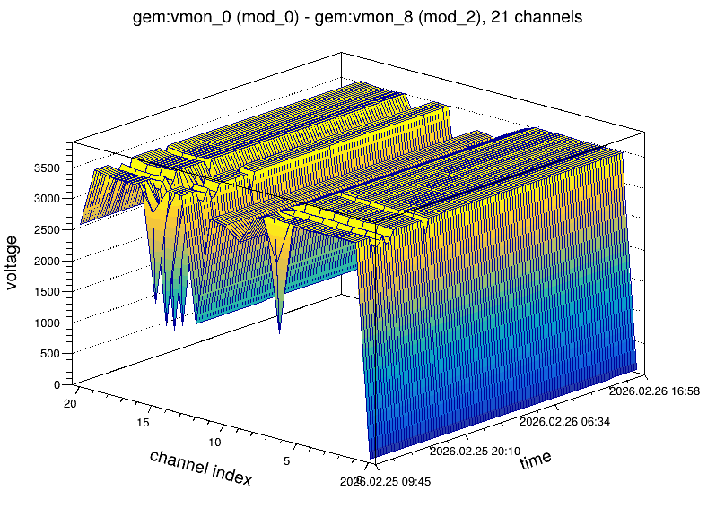
Figure 16. High voltage of the GEM channels for the runs 9696–9730 of Run 9

7. Distributed Computing

The development of the distributed computing infrastructure for the BM@N experiment is required primarily because of the high interaction rate and the large volume of the recorded data. For example, in the Xe run of 2026 (Run 9) with the beam energies of 1.6, 2.2 and 3.0 GeV per nucleon and the Sn and CsI targets, the beam intensity reached 1.6·10⁶ Xe ions per 6-second spill (at 2.2 GeV per nucleon), the trigger rate was up to 20 thousand events per spill (about 1 700 events per second on average), the DAQ system delivered up to 2 GB/s of raw data (800 MB/s on average per run), and the size of a raw BM@N event was about 540 KB. During the session, which lasted from February 12 to April 4, 2026, more than 2.9·10⁹ physics events were collected, and the total raw data amount to 1.8 PB in about 236 thousand files to be stored and processed. Figure 17 shows the general scheme of the data processing pipeline from the data acquisition to the distributed processing and storage, including archival storing.

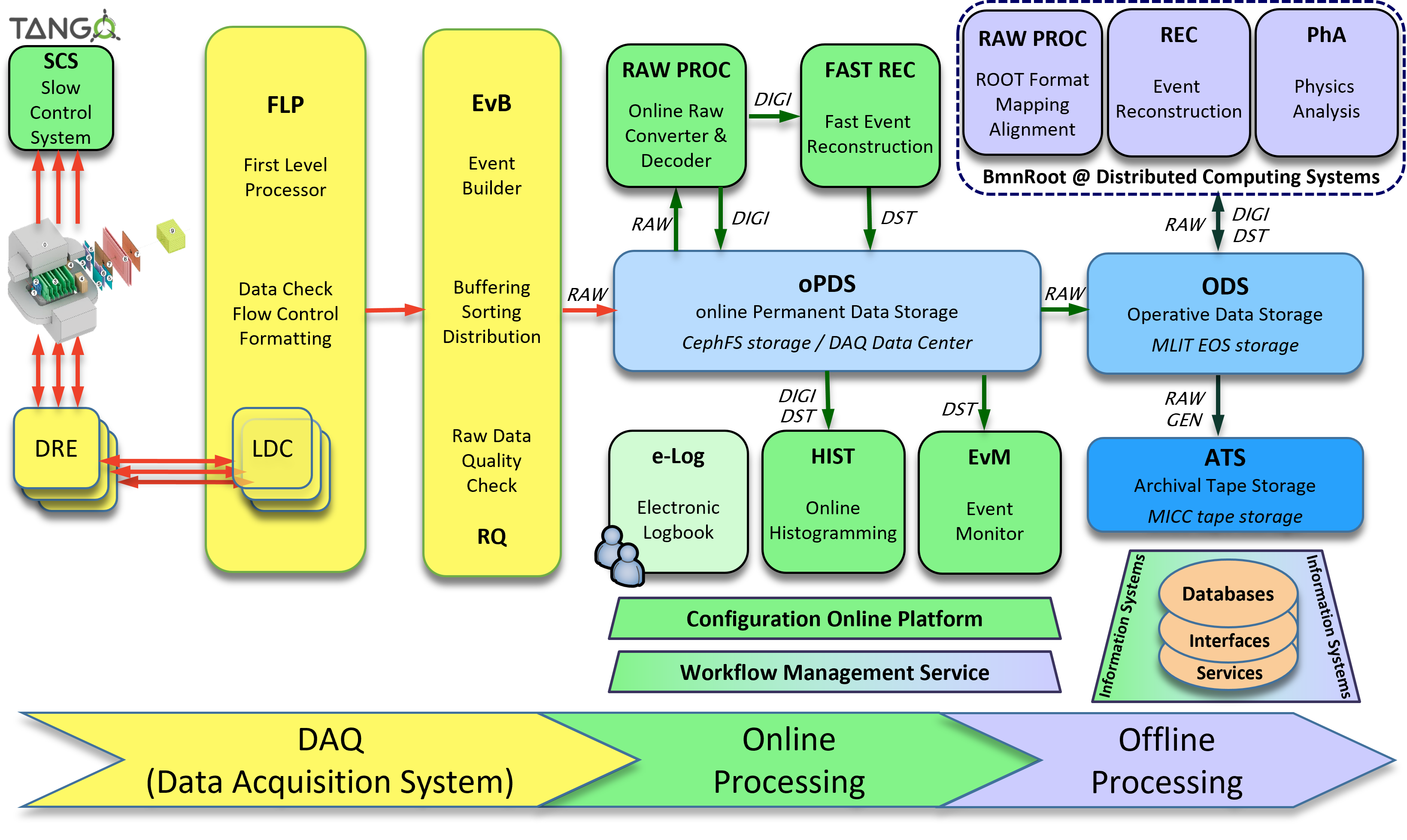
Figure 17. Data processing pipeline

The BM@N data are stored and processed on several computing platforms of JINR: the DAQ Data Center (DDC) of the experiment, the NICA cluster (NCX), the Central Information and Computing Complex (CICC) of the Meshcheryakov Laboratory of Information Technologies (MLIT), and the HybriLIT heterogeneous platform with the Govorun supercomputer. All the platforms use the SLURM batch system, provide access to the BM@N data on the EOS distributed storages – on the NICA cluster and in the MICC complex of MLIT (Section 7.5), and the necessary software – BmnRoot, FairSoft and FairRoot – is available there via the CVMFS repository /cvmfs/bmn.jinr.ru.

After the login to any of the computing platforms, the cluster_config.sh file corresponding to the platform has to be executed in the terminal to set the environment variables for the work, e.g. on the platforms with AlmaLinux 9:

source /cvmfs/bmn.jinr.ru/config/x86_64-alma9/cluster_config.sh

On the NICA cluster with CentOS 7, the x86_64-centos7 directory is used instead of x86_64-alma9. FairSoft, FairRoot and BmnRoot are already installed on the clusters in the CVMFS file system, therefore, to develop and use your own version of BmnRoot, it is enough to install BmnRoot in your directory (Section 2.3), not forgetting one of the installation steps “source SetEnv.sh”, since the paths to the actual versions of FairSoft and FairRoot are also set by the cluster_config.sh file.

The main parameters of the computing platforms are summarized in the table below, and the following subsections briefly describe the platforms with the references to the short instructions on the BM@N website.

Platform	Login	OS	Batch system	EOS storage with BM@N data
DAQ Data Center (DDC)	ddc.jinr.ru (ddc[01-02])	AlmaLinux 9	SLURM	/eos/lpp/nica/bmn/ (NCX EOS) /eos/lit/nica/bmn/ (MICC EOS)
NICA cluster (NCX)	ncx.jinr.ru (ncx[101-106])	CentOS 7	SLURM	/eos/nica/bmn/
MLIT CICC complex	lxui.jinr.ru (lxui[10-11])	AlmaLinux 9	SLURM	/eos/nica/bmn/
HybriLIT platform with the Govorun supercomputer	hydra.jinr.ru	AlmaLinux 9	SLURM, incl. the bmn queue (192 cores)	/eos/eos.jinr.ru/nica/bmn/ (MICC EOS) /eos/eosnica.jinr.ru/nica/bmn/ (NCX EOS)

7.1 BM@N DAQ Data Center

The online DAQ Data Center (DDC) of the BM@N experiment receives the data from the Data Acquisition System and acquires information for monitoring and diagnostics of the main units and detectors of the experiment. Between the Nuclotron sessions, its computing nodes are partially idle and can be used for offline data processing. To work on the DDC, an approval of the BM@N leader is required, as well as a JINR SSO account and an account of the JINR CICC complex, which is used to log in to the interactive machine:

ssh [username]@ddc.jinr.ru

The DDC provides the SLURM batch system with the common batch queue (Intel Xeon cores). Besides the home directory, which should not be used for parallel processing, the users have the Ceph space /ceph/bmn/work/[username] as a faster storage for temporary results, and their directories on the EOS storages of the NICA cluster and MLIT mounted at /eos/lpp/nica/bmn/users/[username] and /eos/lit/nica/bmn/users/[username]. The brief instruction on working with the DDC is given on the BM@N website: https://bmn.jinr.int/bmn-daq-computing-center/.

7.2 NICA Cluster

The offline computing NICA cluster for the experiments of the NICA project was launched at the Veksler and Baldin Laboratory of High Energy Physics in 2019. The NICA cluster consists of two parts: the interactive part, which can be connected to and interactively used by users, and the batch part, where the user jobs are executed in parallel by the SLURM batch system.

The interactive machines of the NICA cluster (ncx[101-106].jinr.ru) are available for the users of the NICA collaborations. To log in, use your account, e.g.:

ssh -X [username]@ncx.jinr.ru

Users connecting to any interactive machine of the NICA cluster are directed to the same home directory /lhep/users/$USER, which space is limited to 50 GB. For your data, you can use the directory on the NCX EOS storage (/eos/nica/bmn/users/$USER, it is created on request with a desired space size to the software coordinator, gertsen@jinr.int), the scratch spaces /scratch1, /scratch2 and /scratch3, as well as the fast temporary storages /junk and /scratch on SSD disks, where files are automatically deleted if they have not been accessed for a while (4 days for /junk, 2 weeks for /scratch).

The rules of using the NICA cluster and the brief instruction on working with it, including the setting of the BmnRoot environment, are given on the BM@N website: https://bmn.jinr.int/how-to-use-the-nica-cluster/.

7.3 MLIT Central Information and Computing Complex

The JINR Central Information and Computing Complex (CICC) of MLIT is constructed as a uniform information resource for all projects with the JINR participation. The CICC cluster machines are available for the NICA users: once the account is registered by the CICC administrators, you can log in to the interactive lxui.jinr.ru (lxui[10-11].jinr.ru) machines, e.g.:

ssh [username]@lxui11.jinr.ru

The CICC provides the SLURM batch system with common queues, such as the cicc queue. The users have the home directory /afs/jinr.ru/user/[username], the NICA user directory on the CICC EOS storage /eos/nica/bmn/users/[username] and the local scratch space /scr/u/[username]. The brief instruction on working with the CICC complex is given on the BM@N website: https://bmn.jinr.int/jinr-cicc-complex/.

7.4 HybriLIT Platform with the Govorun Supercomputer

The HybriLIT heterogeneous platform is a computational component of the Multifunctional Information and Computing Complex (MICC) of MLIT for data processing and analysis, which includes the Govorun supercomputer consisting of a multi-core component and computation accelerators (Intel Xeon Phi co-processors and NVIDIA graphics cards). After the registration in the HybriLIT complex, you can log in with your account:

ssh [username]@hydra.jinr.ru

The platform provides a minimal OS installation, therefore some system packages have to be loaded after the login before setting the BmnRoot environment, as described in the instruction for the platform.

The SLURM batch system of the platform provides several partitions (queues), and the Govorun supercomputer provides common queues, e.g. cascade with Intel Xeon processor cores, volta and ampere with NVIDIA GPU cards. Furthermore, there is a special queue for the BM@N experiment with 192 Intel Xeon cores – bmn (add the “-p bmn -q bmn” parameters to your job description). The user home directory (100 GB quota) is intended for editing files and building programs, whereas the working directory /lustre/projects/[a-z]/[username] is used for computations and data storage; the EOS storages of MLIT and of the NICA cluster are mounted at /eos/eos.jinr.ru/nica/bmn/ and /eos/eosnica.jinr.ru/nica/bmn/. The brief instruction on working with the platform is given on the BM@N website: https://bmn.jinr.int/hybrilit-govorun-sc/.

7.5 Distributed Data Storage

The EOS distributed file system developed at CERN is used to organize the data storage of the BM@N experiment. EOS aggregates the disks of the storage servers in a common distributed file system, and automatic replication and self-checking services working as background processes make it possible to prevent data loss and to restore files in case of hardware or software failures. Two EOS storages are used for the BM@N data: the storage of the NICA cluster (NCX EOS) and the central EOS storage of the MICC complex of MLIT (MICC EOS).

The BM@N experimental and simulated data are located in the exp and sim directories of the EOS storages: /eos/nica/bmn/exp/ and /eos/nica/bmn/sim/ on the NICA cluster and the CICC complex. Both storages are mounted on the computing platforms, though the mount paths differ (see the table at the beginning of the section).

In addition to the mounted spaces, the EOS data can be accessed from any place by the XRootD and EOS protocols: the xrdcp and eos cp commands copy EOS files, and the root://ncm.jinr.ru/ (NCX EOS) and root://eos.jinr.ru/ (MICC EOS) prefixes allow opening remote EOS files directly in the ROOT environment, e.g.:

TFile* f = TFile::Open("root://ncm.jinr.ru//eos/nica/bmn/exp/<file>.root");

To parallelize the data processing on the computing platforms, batch systems are used to distribute user jobs on the cluster nodes, and the NICA-Scheduler has been developed to simplify their usage for the BM@N data processing.

7.6 Batch Systems for Distributed Job Execution

If you have time-consuming tasks, many simple tasks or a lot of files to process, you can use the batch systems of the computing platforms to essentially accelerate your work. A batch system combines the computing nodes of a cluster into a pool of workers, queues user jobs and runs them on free processor slots. The SLURM batch system is used on all the computing platforms described above.

If you know how to work with SLURM, you can submit your jobs directly by the sbatch command. For example, a simple SLURM job script running the reconstruction of a simulated file with the BmnRoot installation from CVMFS can look as follows:

#!/bin/bash
#SBATCH -J bmn_reco          # job name
#SBATCH -n 1                 # number of tasks
#SBATCH --mem-per-cpu=4G     # memory per processor
source /cvmfs/bmn.jinr.ru/bmnroot/dev/x86_64-alma9/bmnroot_config.sh
cd /eos/nica/bmn/users/ivanov
root -b -q '$VMCWORKDIR/macro/run/run_reco_bmn.C("bmnsim.root", "bmndst.root")'

The job is submitted by the command “sbatch reco_job.sh”. However, writing job scripts for many input files, splitting the processing into parallel tasks and merging the results require additional effort. To simplify parallel processing of the BM@N data without knowledge of batch systems, the NICA-Scheduler has been developed.

7.7 NICA-Scheduler

NICA-Scheduler is a module package developed for the FairRoot-based frameworks, such as BmnRoot. It is included in BmnRoot as the services/nica_scheduler submodule and is built together with it. NICA-Scheduler uses an existing batch system (SLURM, SGE and Torque are supported) to distribute user jobs on a cluster, and also supports multithreaded execution on a local multicore machine. Jobs for distributed execution are described in XML files and passed to the scheduler:

nica-scheduler my_job.xml

The description of a job starts with the <job> tag. The <macro> tag sets a ROOT macro to be executed and, optionally, the start event and the number of events to process. The <file> tags inside it define input files – a file path, a mask with wildcards, a text list of files, the result files of a previous macro or job, or a list of files selected from the Unified Condition Database – and the result files; special variables, e.g. ${counter}, ${file_name} or ${user}, can be used to form their names. The <run> tag sets the execution mode (‘global’ – on a cluster with the batch system, ‘local’ – on the user machine, ‘container’ – on a cluster in a container environment), the maximum number of processors for the job, the configuration scripts setting the environment (e.g. config.sh of BmnRoot) and other resources. An arbitrary command can be executed by the <command> tag instead of a ROOT macro. Several macros can be chained in one job, and several jobs with dependencies can be combined by the <jobs> tag.

Example of a job running the simulation of DCM-SMM files and the reconstruction of the simulated events on the NICA cluster with 30 processors:

<job>
 <macro name="bmn_sim" path="$VMCWORKDIR/macro/run/run_sim_bmn.C"
        start_event="0" event_count="0" add_args="DCMSMM">
  <file input="/eos/nica/bmn/sim/gen/DCMSMM/DCMSMM_XeCsI_3.9AGeV_mb_10k/*_116*"
        output="/eos/nica/bmn/users/${user}/bmnsim_${file_name}.root"/>
 </macro>
 <macro name="bmn_reco" path="$VMCWORKDIR/macro/run/run_reco_bmn.C"
        start_event="0" event_count="0">
  <file macro_input="bmn_sim"
        output="/eos/nica/bmn/users/${user}/bmndst_${file_name:~7}.root"/>
 </macro>
 <run mode="global" count="30"
      config="/cvmfs/bmn.jinr.ru/bmnroot/dev/x86_64-alma9/bmnroot_config.sh"/>
</job>

NICA-Scheduler can also parallelize the processing of one input file: the parallel_mode attribute of the <file> tag sets the number of processors to process parts of the file, and the merge attribute defines whether the partial results are merged into one result file.

The detailed description of the NICA-Scheduler with all XML tags and attributes is given in the services/nica_scheduler/README.md file, and the services/nica_scheduler/examples directory contains various XML examples of jobs for the BM@N data processing.

8. BmnRoot Development

BmnRoot is developed by the members of the BM@N collaboration in the GitLab repository of JINR. This chapter describes the work with the Git version control system, the automatic testing and deployment of new versions of BmnRoot, and the coding conventions.

8.1 Using Git

The source code of BmnRoot is managed by the Git version control system. The main development branch of the repository is dev, and the stable versions of BmnRoot are fixed by tags and releases. This section describes the access to the repository and the use of Git in the development of BmnRoot.

The repository is open for reading: the latest development version of BmnRoot can be cloned with HTTPS without registration and SSH keys, or downloaded as a ZIP archive, which, however, does not include the submodules of the repository, e.g. the interfaces of the databases:

git clone -b dev --recursive https://git.jinr.ru/nica/bmnroot.git

To make changes, register on the JINR GitLab with an e-mail of JINR or send a request with a short description of your work and the preferred login to the software coordinator (gertsen@jinr.int). Then add an SSH key to your GitLab profile (see the instruction on generating the key), so that the password is not asked at every access to the repository. Set your name and e-mail, since every commit uses them to identify you as the author; the last command shows the entered values together with the other global options of Git:

git config --global user.name "YOUR_NAME"
git config --global user.email "your_email@example.com"
git config --global --list

Clone the repository with SSH together with its submodules:

git clone -b dev --recursive git@git.jinr.ru:nica/bmnroot.git

In the directory of the repository, the first command below downloads the latest changes of the current branch and of the submodules (for Git versions earlier than 2.14, use “git pull && git submodule update --init” instead), the second one lists all the branches of the repository on the server, and the third one switches to an existing branch to work on it:

git pull --recurse-submodules
git branch -r
git checkout NAME-OF-BRANCH

Direct changes of the main branches of BmnRoot, such as dev, are not possible: the branches are protected. A developer makes the changes in an own branch and brings them into a main branch by a merge request of the own branch. The branch is created from the latest version of dev and named after the task for common understanding, e.g. feature-new-geometry or bugfix-old-problem (a name cannot contain spaces, so hyphens or underscores are used instead):

git checkout dev
git pull --recurse-submodules
git checkout -b feature-new-geometry

Git keeps track of the added, changed and deleted files and folders. The first command below shows the status of the changes: the changed files and the files added to the staging area, i.e. to the next commit. The second one shows the differences between the local changes, which are not added to the staging area yet, and the version of the repository that you cloned or pulled:

git status
git diff

The new or changed files and folders are added to the staging area, committed to the local repository with a short description of the changes, and the commits of the own branch are pushed to the GitLab repository (the origin remote):

git add <changed files>
git commit -m "Short description of the changes"
git push origin feature-new-geometry

Then a merge request of the own branch into the main branch (e.g. dev) is created on the Merge requests page of the repository. For every merge request, the GitLab CI tests the new version of BmnRoot: the formatting of the changed files is checked (Section 8.2), BmnRoot is built for the supported operating systems, and the main macros of the simulation, raw data decoding and reconstruction are run on test data. The changes are merged into the main branch only if the testing is successful: then the merge request is merged by the Merge button on its page. Otherwise, the errors are fixed in the own branch, and the new commits pushed to it update the merge request and start the testing again. In addition, all the macros of BmnRoot are run regularly, and their status is published on the BM@N website in the ‘Software – BmnRoot – Macro Status’ section.

Every new version of the dev branch, as well as the tags and releases, is deployed to the CVMFS repository of the experiment automatically: the installations for the supported operating systems are placed to /cvmfs/bmn.jinr.ru/bmnroot/<branch or tag>/x86_64-<OS>, e.g. /cvmfs/bmn.jinr.ru/bmnroot/dev/x86_64-alma9 (Section 7). At the same time, new containers with BmnRoot are built, and the Doxygen reference documentation of BmnRoot is generated. The tags and releases are created by the software coordinator of the experiment; their names have the YY.MM.P form, e.g. 26.10.0, where P is the patch number of the release (Section 6.2.1).

Besides the command line, Git can be used with graphical tools. Most code editors and development environments have built-in Git support, which is now the most common way to use Git. For example, the Source Control view of VS Code shows the changed files and their differences, adds the changes to the staging area, commits them, creates and switches branches, and pulls and pushes the commits. The GitLab Workflow extension of VS Code shows the merge requests and the status of the GitLab CI pipelines in the editor; it is connected to the JINR GitLab with a personal access token with the api scope. On Linux, the standalone graphical clients git-cola and gitg are popular, and the simple gitk and git gui tools are part of Git (some Linux distributions provide them as separate packages). On Windows, Git is installed as Git for Windows, which is also used by VS Code. Other graphical clients for all platforms are listed on the Git website.

The complete Git documentation is given in the Pro Git book (also in Russian), and the Git How To tutorial (also in Russian) introduces Git step by step.

8.2 Coding Conventions

The coding conventions make the code written by many developers uniform, so that it is easy to read, review and maintain. New code follows these conventions, and the changed parts of old code are brought to them.

The C++ code of BmnRoot is formatted according to the current rules of the clang-format tool given in the .clang-format file in the top directory of the repository. The format is based on the Mozilla style with the following main rules: indentation by 4 spaces without tabs, lines up to 120 characters, the opening brace of a class, structure, enumeration, namespace or function on a new line, the pointer and reference signs next to the type (int* p), and grouped and sorted #include directives.

When changes are brought into the main branches of the BmnRoot repository in GitLab, the check of the code formatting is mandatory: the GitLab CI checks the C++ files changed in a merge request with clang-format. If some of them are not formatted, the testing fails, and the merge request gets the ‘Unformatted’ label and a comment with the command formatting these files. Therefore, the changed files should be formatted before the commit:

clang-format -i --style=file <changed files>

The check uses clang-format 19, and other versions of the tool can format some code differently, so the same version is recommended, e.g. from the CVMFS repository of CERN:

source /cvmfs/sft.cern.ch/lcg/releases/clang/19.1.3-e838d/x86_64-el9/setup.sh

Most code editors and development environments (e.g. VS Code, CLion, Qt Creator) can format the code with the .clang-format file automatically, for instance, when a file is saved.

BmnRoot follows the naming conventions of ROOT and FairRoot. Names are meaningful: abbreviations are used only if they are commonly accepted, such as MC, TOF or DST.

• Class names start with the Bmn prefix and are written in the CamelCase style, e.g. BmnGemStripHit. The name contains the detector or subsystem and the role of the class, for which the common suffixes are used: Point (MC points), Digit, Hit and Track for the data classes, Digitizer, HitProducer or HitMaker and Finder for the tasks, Raw2Digit for the converters of the raw data, Qa for the quality assurance. The interfaces of the information systems have their own prefixes, e.g. UniRun of the Condition Database, and the classes taken from the CBM experiment keep the Cbm prefix.
• Functions start with an uppercase letter and usually with a verb, e.g. FindTracks() or IsSelected(). The getter and setter of a data member fX are named GetX() and SetX(), e.g. GetNHits() and SetMinCharge().
• Data members start with f followed by a capitalized word, e.g. fNHits; static data members start with fg (fgk for static constants).
• Constants and enumeration values start with k, e.g. kGEM of BmnDetectorList.h.
• Local variables and function arguments start with a lowercase letter, e.g. nHits for a number of hits and iHit for the loop index over the hits.
• The files of a class are named after the class, e.g. BmnGemStripHit.h and BmnGemStripHit.cxx. The main macros are named in lower case with underscores, e.g. run_reco_bmn.C.

The code has to be commented, and the comments and the documentation are written in English. The comments are concise and meaningful: they explain the “why” behind complex logic, e.g. the reason for an algorithm, a correction or a selection cut, rather than repeating what is obvious from the code. Ordinary comments (//) explain the implementation in the source (.cxx) files, and Doxygen comments describe the classes and functions in the header (.h) files.

The reference documentation of BmnRoot is generated by Doxygen from the comments in the source code and from the README.md files of the directories after every change of the dev branch, and it is published at http://nica.pages.jinr.ru/bmnroot. The rules of the documentation are given on its Code Documentation Rules page (the services/doxygen/documentation_rules.md file of the repository); the main of them are the following:

• New classes, their public functions and data members are documented in the header (.h) files with the Doxygen comments: /** ... */ or /// before a declaration and ///< after a data member on the same line.
• A description starts with a short sentence, which is shown in the lists of classes and members. The parameters and the return value of a function are described with @param and @return, including the units of physical quantities and the owner of a returned object.
• Transient data members, which are not written to ROOT files, are marked with ///<!, not with //!, whose comment Doxygen attaches to the next member.
• Every directory with code has a README.md file with the description of the directory and the tables of its classes, files and subdirectories.
• Unused code is deleted rather than commented out, since Git keeps the history of all changes.

For example, the description of a function and of the data members in a header file:

/**
 * Fits the track with the Kalman filter.
 * @param track track to fit, its parameters are updated
 * @param pdg PDG code of the particle hypothesis
 * @return chi2 of the fit, or a negative value if the fit failed
 */
Double_t FitTrack(BmnTrack* track, Int_t pdg = 211);
 
Int_t fNHits;          ///< number of hits
TClonesArray* fHits;   ///<! input hits, not stored

The code of BmnRoot is organized by the following rules. Each part of the code is placed according to its purpose (Section 3.1): the code of a detector, e.g. its geometry, digitization and hit reconstruction, is in its directory of detectors, the tracking and global reconstruction – in reconstruction, the physics analysis – in physics, the data classes used by several packages – in base/data, and the macros – in macro.

• A directory is built into a library: its CMakeLists.txt file contains the list of the source files, and its LinkDef file – the classes of the ROOT dictionary. A new class is added to both (Section 9.1) and described in the README.md file of the directory.
• Each class has its own pair of files: the header (.h) with the declaration and the source (.cxx) with the implementation. The header is protected from repeated inclusion by an include guard (#ifndef BMNGEMSTRIPHIT_H, #define BMNGEMSTRIPHIT_H … #endif).
• The headers of the used classes are included explicitly; forward declarations (class X;) are used only to break circular dependencies between headers.
• A class with the ROOT dictionary has the ClassDef (or ClassDefOverride) macro with the version of the class. The version is increased when the data members of a class written to files change, so that ROOT can still read the files written before.
• Deep nesting of loops and conditions is avoided, since it makes the code hard to read and test. The nesting is reduced by early exits, e.g. if (!hit) continue; or return in case of an error, and by moving the inner parts of the code into separate functions.
• Parameters, calibrations and geometry constants are not hard-coded: they are taken from the databases (Section 6), the geometry or the configuration files of the config directory.
• The repository contains the source code and the small input files needed by the software: data files (e.g. ROOT files), build results and personal test files are not committed.

The DRY (Don't Repeat Yourself) principle requires that every piece of knowledge, i.e. an algorithm, a constant or a parameter, is implemented in one place of the code. Copied code has to be changed and fixed in all its copies, which is easily forgotten: the copies diverge, and the errors remain in some of them. In BmnRoot, it means the following:

• Before writing new code, look for an existing implementation in the Doxygen documentation and in the README.md files. For instance, the data classes of all processing levels are in base/data, the mathematical tools (fits, Kalman filter, matrix operations, material effects) – in base/math, helper functions (file checks, input file lists, magnetic field by the beam energy) – in BmnFunctionSet, the detector identifiers – in BmnDetectorList, and the common enumerations – in BmnEnums.h.
• Code common to several classes, e.g. to similar detectors or tasks, is moved to a base class or a common function instead of being copied. An existing class is extended, e.g. by a new parameter or mode, rather than copied under a new name.
• A constant is defined once, e.g. as a constant of a class or in BmnEnums.h, and a parameter is read from its single source, a database or a configuration file, instead of repeating the number in several places.
• When an existing task is copied as the starting point of a new one (Section 9.1), the code not needed by the new task is removed.

9. Frequently Asked Questions

9.1 How to create a new task, e.g. for physics analysis?

A new task, e.g. an analysis task for run_ana_bmn.C or a reconstruction task, can be created in two ways:

1. Using the FairRoot template (recommended). The NewTask template of FairRoot (Section 2.2) contains the skeleton of a task derived from FairTask with the main functions: SetParContainers() to request the parameter containers, Init() to get the input branches from FairRootManager and to register the output ones, Exec() called for every event, ReInit() called when the run changes, and Finish() called at the end of the run. Copy the template directly to the directory, where the task will be implemented, e.g. to a new subdirectory of physics for an analysis task, and rename the files and classes by the script, which takes the name of the task (the script processes all the source files of the current directory, therefore a separate subdirectory is used):

   cp -r <FairRoot source>/templates/NewTask $VMCWORKDIR/physics/myana
   cd $VMCWORKDIR/physics/myana
   ./rename.sh BmnMyAnalysis
   rm rename.sh

2. Copying an existing task. Any existing task, which is the most suitable for the purpose, can be copied, renamed and modified, for example, the BmnAnalysisTask class (physics/BmnAnalysisTask.h and .cxx), which is a template of an analysis task in BmnRoot, or BmnTwoParticleDecay (physics/decay), which is an example of a complete analysis task. This way quickly gives a working task, but it also copies the code specific for the original task, which has to be carefully cleaned.

Then add the new source file to the list of sources in the CMakeLists.txt file of the library (e.g. physics/CMakeLists.txt, also with the new subdirectory in the include directories) and the class to its LinkDef file (e.g. physics/PhysicsLinkDef.h), rebuild BmnRoot, and add the task to the corresponding macro: an analysis task – to the “Analysis Tasks” block of run_ana_bmn.C (Section 4.6), a reconstruction task – to run_reco_bmn.C (Section 4.5), and a task of the simulation, e.g. a digitizer, – to run_sim_bmn.C (Section 4.3). For example, for the analysis task created above:

# physics/CMakeLists.txt: the source file in the set(sources ...) list
myana/BmnMyAnalysis.cxx
# and the subdirectory in target_include_directories(...)
$<BUILD_INTERFACE:${CMAKE_CURRENT_SOURCE_DIR}/myana>
// physics/PhysicsLinkDef.h
#pragma link C++ class BmnMyAnalysis + ;
// run_ana_bmn.C
BmnMyAnalysis* my_analysis = new BmnMyAnalysis();
fRunAna->AddTask(my_analysis);

9.2 How to add a new detector to BmnRoot?

A new detector for the Monte Carlo simulation can be created in two ways:

1. Using the FairRoot template (recommended). The NewDetector_root_containers template of FairRoot (Section 2.2) contains the skeleton classes of a detector: the detector class derived from FairDetector, which processes the steps of particles in the sensitive volumes and stores MC points (NewDetector), the MC point class (NewDetectorPoint), the geometry interface (NewDetectorGeo, NewDetectorGeoPar) and the parameter container factory (NewDetectorContFact). Copy the template to a new subdirectory of the detectors directory and rename the classes by the script, which takes the detector name, the project name and the prefix of the class names, e.g.:

   cp -r <FairRoot source>/templates/NewDetector_root_containers \
         $VMCWORKDIR/detectors/mydet
   cd $VMCWORKDIR/detectors/mydet
   ./rename.sh BmnMyDet BmnRoot Bmn

2. Copying an existing detector (less recommended way). A detector with a similar structure, e.g. detectors/hodo, is copied to a new directory, and its classes, files and library are renamed. This way quickly gives a working detector, but it also copies the code specific for the original detector, which has to be carefully cleaned.

In both cases, the following steps are required to use the new detector in BmnRoot:

• add the identifier of the detector (k<Name>) to the DetectorId enumeration in base/BmnDetectorList.h before kNOFDETS, and use the CbmStack class (base/data) to add the MC points to the stack of the MC tracks instead of the stack class set by the template;
• add the new directory to detectors/CMakeLists.txt, prepare the CMakeLists.txt and LinkDef files of the detector library similar to the other detectors, so that the classes are built and visible from the ROOT macros;
• prepare the detector geometry in ROOT format, e.g. by a macro similar to the ones of the macro/geometry directory, where the names of the sensitive volumes correspond to the ones processed by the detector class;
• add the detector to the setup: for tests – by the <addSetupModule> element of an XML file with a local customization of the setup (Section 6.2.3), and after the validation – as a new module in the Geometry Database;
• implement a digitizer task converting the MC points into the detector digits and add it to run_sim_bmn.C, and add the corresponding reconstruction tasks to run_reco_bmn.C; the new tasks can be started from the NewTask template of FairRoot.

9.3 How to get full geometry (gGeoManager) of the BM@N facility?

1. In a stand-alone macro from a simulation or DST file (e.g. bmnsim.root or bmndst.root):

   TFile* f = new TFile("bmnsim.root");
   f->Get("FairGeoParSet");
   gGeoManager…

2. In any task executed by FairRunAna:

   // the geometry is already loaded in fRunAna->Init() before Init() of the tasks
   TGeoNode* node = gGeoManager->FindNode(x, y, z);

3. For an existing BM@N run from the Geometry Database (latest approved setup of the period):

   GeoSetup gSetup;
   string tag = gSetup.GetLastApprovedSetupTag("run9");
   // or a tag, e.g. "run9_26.09.0"
   gSetup.LoadSetupToGeoManager(tag);
   gGeoManager…

9.4 How to get magnetic field value?

The magnetic field is set for FairRunAna by the run_reco_bmn.C and run_ana_bmn.C macros (in the analysis – by the information of the DST file), so you can access the magnetic field in any task directly:

FairField* field = FairRunAna::Instance()->GetField();

The value of the magnetic field in the space point can be obtained by any of the following methods:

field->GetBx(x,y,z);
field->GetBy(x,y,z);
field->GetBz(x,y,z);
Double_t point[3], b[3];
field->GetFieldValue(point, b);

Outside FairRunAna, the magnetic field of the run can be created from a DST file:

Double_t fieldScale;  Int_t fieldType;
FairField* field =
    BmnFunctionAna::GetDSTField("bmndst.root", fieldScale, fieldType);

9.5 How to check if the current MC track created hit into active volume of your detector?

Each MC track stores the number of MC points, which the track produced in every detector. You can use the function:

Int_t CbmMCTrack::GetNPoints(DetectorId detId);

for such a check, for example:

FairRootManager* ioman = FairRootManager::Instance();
pMCTracks  = (TClonesArray*) ioman->GetObject("MCTrack");
 
mcTrack = (CbmMCTrack*) pMCTracks->UncheckedAt(mcTrackIndex);
if (mcTrack->GetNPoints(kTOF))
{
     // do your analysis of this track
}

The constant numbers (DetectorId) of all BM@N detectors are described in the header:

bmnroot/base/BmnDetectorList.h